"What I cannot create, I do not understand." -- Richard Feynman

Let's say we want to build a model to discriminate the following red, green and blue points in 2-dimensional space:

import numpy as np
import matplotlib.pyplot as plt
plt.style.use('classic')
np.set_printoptions(precision=3, suppress=True)

X = np.array([[-0.1, 1.4],
              [-0.5, 0.2],
	      [ 1.3, 0.9],
	      [-0.6, 0.4],
	      [-1.6, 0.2],
	      [ 0.2, 0.2],
	      [-0.3,-0.4],
	      [ 0.7,-0.8],
	      [ 1.1,-1.5],
	      [-1.0, 0.9],
	      [-0.5, 1.5],
	      [-1.3,-0.4],
	      [-1.4,-1.2],
	      [-0.9,-0.7],
	      [ 0.4,-1.3],
	      [-0.4, 0.6],
	      [ 0.3,-0.5],
	      [-1.6,-0.7],
	      [-0.5,-1.4],
	      [-1.0,-1.4]])

y = np.array([0, 0, 1, 0, 2, 1, 1, 1, 1, 0, 0, 2, 2, 2, 1, 0, 1, 2, 2, 2])
Y = np.eye(3)[y]
colormap = np.array(['r', 'g', 'b'])

def plot_scatter(X, y, colormap, path):
   plt.grid()
   plt.xlim([-2.0, 2.0])
   plt.ylim([-2.0, 2.0])
   plt.xlabel('$x_1$', size=20)
   plt.ylabel('$x_2$', size=20)
   plt.title('Input 2D points', size=18)
   plt.scatter(X[:,0], X[:,1], s=50, c=colormap[y])
   plt.savefig(path)

plot_scatter(X, y, colormap, 'image.png')

plt.close()
plt.clf()
plt.cla()

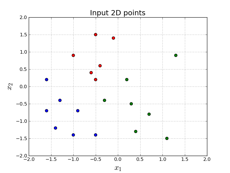
In other words, given a point in 2-dimensions, $\mathbf{x} = (x_1, x_2)$, we want to output either red, green or blue.

We can use Softmax Regression for this problem. We first learn weights, $w_{1,1}, w_{1,2}, w_{2,1}, w_{2,2}, w_{3,1}, w_{3,2}$, and bias, $b_1, b_2, b_3$. This phase is called training. And then, we will use those weights and the bias to predict a new point, $\mathbf{x}$.

We will use Softmax Regression or sometimes called Multinomial logistic regression to solve this problem. This is a simple generalization of Logistic Regression (binary) to arbitrary number of classes.

We represent the output as a one hot vector. In other words, we represent red points using $\begin{bmatrix} 1 \\ 0 \\ 0 \end{bmatrix}$, similarly for green points using $\begin{bmatrix} 0 \\ 1 \\ 0 \end{bmatrix}$, and lastly for blue points using $\begin{bmatrix} 0 \\ 0 \\ 1 \end{bmatrix}$.

Here is a visual representation of our model:

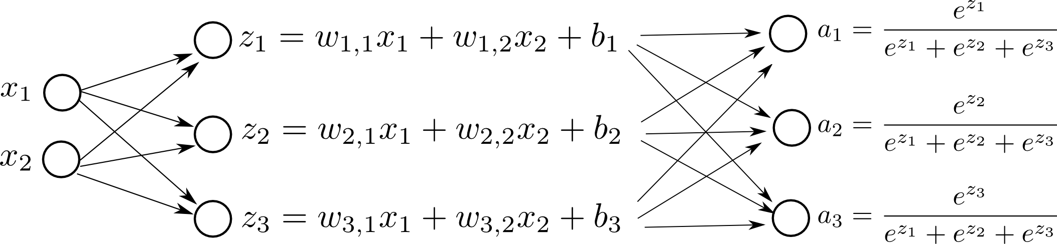
and we simply pick the biggest $a_i$ as our final prediction.

The parameters of our Softmax Regression model are:

So, our goal is to learn these parameters.

We are given the coordinates of the input points in the matrix $\mathbf{X}$ of size $(20 \times 2)$ and their corresponding class labels in $\mathbf{y}$ which is a vector of size $20$.

First, let's assume that we are given the weights, $\mathbf{W}$, and, bias, $\mathbf{b}$. How do we calculate the output?

We represent $\mathbf{X}$ as a matrix. $\mathbf{X}$ contains all the points. In our case $\mathbf{X}$ contains $m=20$ samples and for each sample we have $(\mathbf{x},y)$. $\mathbf{y}$ contains all the labels (red, green and blue). For each of the 20 samples, we have an integer $y^{(i)} \in \{0, 1, 2\}$. We convert $\mathbf{y}$ into a matrix $\mathbf{Y}$ of one hot vectors. $\mathbf{Y}$ is of size $(20 \times 3)$ where each row represents one of the sample's class as a one hot vector.

As we discussed earlier, $\mathbf{W}$ has the weights. $\mathbf{b}$ has the bias. So, to summarize the sizes of the matrices:

• $\mathbf{X}: 20 \times 2$
• $\mathbf{Y}: 20 \times 3$
• $\mathbf{W}: 3 \times 2$
• $\mathbf{b}: 3 \times 1$

Feed-forward basically means: given $\mathbf{x}, \mathbf{y}, \mathbf{W}$ and $\mathbf{b}$, we produce $\mathbf{a}$ and $\text{L}$.

Here is how we do it:

here $\mathbf{x}$ is of size $2 \times 1$. So, $\mathbf{z}$ is of size $3 \times 1$.

After getting $\mathbf{z}$, we apply softmax function to compute $\mathbf{a}$.

\begin{equation} \label{eq:softmax} a_i = \frac{e^{z_i}}{\sum_{j=1}^N e^{z_j}} \end{equation}

A nice property of the Softmax function that it produces a legit Probability Distrubition. In classification (or more generally in Machine Learning) we often want to assign prababilities to categories or classes. Softmax function is known to work well for numereous applications/areas.

Softmax is a vector function -- it takes a vector as an input and returns another vector.

There is an issue with the naive implementation of Softmax function we should keep in mind. The Equation $\ref{eq:softmax}$ may be problematic to compute for big values of $z_i$. We call this phenomena numerically unstable. Because $e^{z_i}$ can easily overflow 64bit (even 128bit). We need to approach this computation slightly differently.

The Softmax function takes an N-dimensional vector of real values and returns a new N-dimensional vector that sums up to $1$. In this tutorial, N is 3. Please see the softmax function in Equation $\ref{eq:softmax}$.

Let's look at an example:

def softmax(a):
  return np.exp(a) / np.sum(np.exp(a))

a = np.array([1.0, 2.0, 3.0])
print a
print softmax(a)

[1. 2. 3.]
[0.09  0.245 0.665]

Intuitively, softmax increases/emphasizes the relative difference between large and small values.

However, we may have numerical stability issues if we naively try to apply softmax function. Let's look at this:

def softmax(a):
  return np.exp(a) / np.sum(np.exp(a))

a = np.array([1000.0, 2000.0, 3000.0])
print a
print softmax(a)

[1000. 2000. 3000.]
[nan nan nan]

We are getting nan values along with a RuntimeWarning: overflow encountered in exp. Simply because:

print(np.exp(1000))

inf

$e^{1000}$ overflows and numpy returns positive infinity. So, both our numerator and denominator becomes inifity, and numpy returns nan for the division.

There is a nice approach to compute the exact same function with a simple math trick:

for some fixed $K \in \mathbb{R}$. And we can pick $K = - max(z_1, z_2, \dots, z_N)$.

So, practically, we compute the same $\mathbf{a}$, using the below code, that does not have the same numerical stability issues we had before:

def softmax(a):
  return np.exp(a-max(a)) / np.sum(np.exp(a-max(a)))

a = np.array([1000.0, 2000.0, 3000.0])
print a
print softmax(a)

[1000. 2000. 3000.]
[0. 0. 1.]

As you can see, we fixed the nan issues with this simple trick.

However, we still have some numerical issues. First and second value of the softmax shouldn't be $0$, they should be very close $0$, but not exactly $0$. But this is good enough for now.

So, to wrap-up the Feed-Forward phase, we can finalize the feed-forward step:

def stable_softmax(z):
  # z is 3 x 1
  a = np.exp(z - max(z)) / np.sum(np.exp(z - max(z)))
  # a is 3 x 1
  return a

def forward_propagate(x, W, b):
  # W is 3 x 2
  # x is 2 x 1
  # b is 3 x 1
  z = np.matmul(W, x) + b
  a = stable_softmax(z)
  # z is 3 x 1
  # a is 3 x 1
  return z, a

W = np.array([[ 0.31, 3.95],
              [ 7.07, -0.23],
              [-6.27, -2.35]])

b = np.array([[ 1.2  ],
              [ 2.93 ],
              [-4.14 ]])

z, a = forward_propagate(X[0,:].reshape(2,1), W, b)

print(z)
print(a)
print(y[0])

[[ 6.699]
 [ 1.901]
 [-6.803]]
[[0.992]
 [0.008]
 [0.   ]]
0

Above, we feed the first sample of our $m=20$ samples. It is a red point, and our classifier produces a one hot vector which confidently says red as well. So, our classifier does a good job for this sample. In fact, this classifier correctly classifies all the samples correctly, so it has 100% accuracy.

So, given the weights, and bias, it is pretty straight-forward to calculate the final prediction. The tricky part is to learn the parameters (weights and the bias) properly.

In training, our goal is to learn a matrix $\mathbf{W}$ of size $3 \times 2$, and a $\mathbf{b}$ of size $3 \times 1$ that best discriminates red, green and blue points.

We want to find $\mathbf{W}$ and $\mathbf{\mathbf{b}}$ that minimizes some definition of a loss function (or cost function). Let's attempt to write a loss function for this problem.

Let's say we have three points:

Now, let's list these $y$ as a one hot vector and, their corresponding imaginary $\mathbf{a}$ values:

Intuitively, we want a classifier that produces similar looking $\mathbf{a}$ and $\mathbf{y}$. This means, if $\mathbf{y} = \begin{bmatrix} 1 \\ 0 \\ 0 \end{bmatrix}$, then, for example, having $\mathbf{a} = \begin{bmatrix} 0.8 \\ 0.1 \\ 0.1 \end{bmatrix}$ is more desirable than having $\mathbf{a} = \begin{bmatrix} 0.6 \\ 0.2 \\ 0.2 \end{bmatrix}$.

One simple way of encoding this intuition using a maximization problem is as follows. We want to maximize:

Here, $a_j$ represents the jth item in the vector $\mathbf{a}$, and similarly $y_j$ represents the jth value in $\mathbf{y}$. For example, when $\mathbf{a} = \begin{bmatrix} 0.9 \\ 0.1 \\ 0.0 \end{bmatrix}$, then, $a_1 = 0.9, a_2 = 0.1$ and $a_3 = 0.0$.

Similar to Logistic Regression, we need to define the loss for multiple samples. We will apply Maximum Likelihood Estimation again, and try to maximize the multiplication for each sample:

here, $y^{(i)}$, $x^{(i)}$ and $a^{(i)}$ corresponds to ith sample in the training set out of $M$ training samples.

Maximizing above is equal to maximizing:

since we like to minimize things instead of maximizing:

If we add our Log Loss to our computation graph, for one sample:

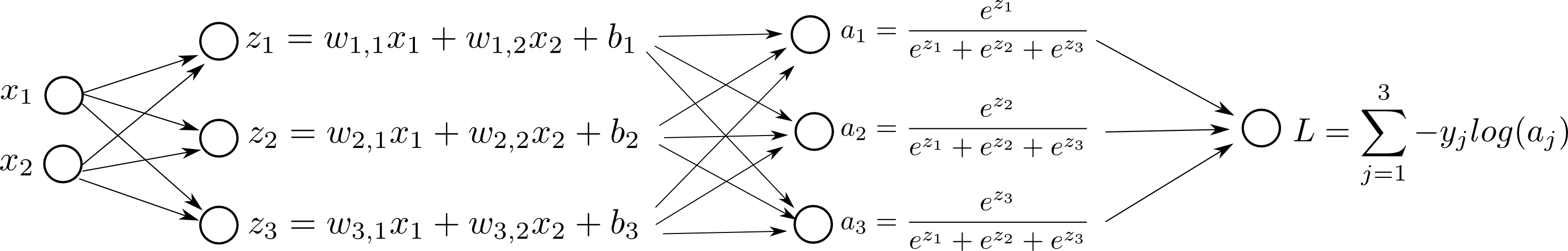
Also, this loss function is sometimes called Cross Entropy Loss Function in some contexts.

We need to be careful when computing the loss function.

Here is the loss function we came up with:

Notice that $y \in \{0, 1\}$ and $0 < a_j < 1$. What are the possible values for $\text{L}$?

We have seen the natural logarithm function in the previous tutorial, and remember that it is not numerically stable for small input values.

So, let's try to: come up with mathematically equal way that is numerically okay.

for some fixed $K \in \mathbb{R}$. And we can pick $K = - max(z_1, z_2, \dots, z_N)$. As we have done before.

This is way better, because we got rid of the first $\text{log}$, and the domain of the second $\text{log}$ function is $[1, \infty )$, hence, it is numerically stable.

We want to start with random parameters and make our parameters better and better gradually as an iterative manner. Gradient descent is simply:

The tricky part here is to compute $\frac{d L}{d \mathbf{W}}$ and $\frac{d L}{d \mathbf{b}}$. We need to do a small scale back propagation of derivatives here.

But first, let's see what happens if we change $w_{2, 1}$ in the network, step by step:

In order to do gradient descent, we need the derivatives, $\frac{d L}{d \mathbf{W}}$ and $\frac{d L}{d \mathbf{b}}$:

Let's write an example for $\frac{dL}{d w_{2,1}}$ explicitly:

Above, we are summing up the contribution of the change of $w_{2,1}$ over different "paths": $a_1, a_2, a_3$. In other words: when we change $w_{2,1}$; $a_1, a_2$, and $a_3$ changes as a result. Then, the change of $a_1, a_2$ and $a_3$ effects $L$. We sum up all the changes $w_{2,1}$ produces over each $a_1, a_2$ and $a_3$ to $L$.

So, we need the derivatives: $\frac{dL}{d a_i}, \frac{da_i}{dz_m}$, $\frac{dz_m}{dw_{m,n}}$ and $\frac{dz_m}{db_m}$.

Let's do some calculus:

Now, we only missing the derivative of the Softmax function: $\frac{d a_i}{d z_m}$.

Softmax is a vector function -- it takes a vector as an input and returns another vector. Therefore, we cannot just ask for the derivative of softmax, we can only ask the derivative of softmax regarding particular elements.

For example,

refers to how much $a_1$ will change if play with $z_2$.

Using the same logic for each element for $a_i$ and $z_j$ would produce us $N \times N$ matrix of derivatives. This is sometimes called a Jacobian matrix. Let's think there is a function $f$ , in this case this is the softmax function, takes an array and returns an array: $f: \mathbb{R}^n \rightarrow \mathbb{R}^m $. The derivative matrix, Jacobian matrix, $\mathbf{J} \in \mathbb{R}^{m \times n}$.

Let's try to take derivative for one particular element:

We can use Quotient Rule here. Recall that:

In our case:

Let's apply Quotient Rule.

if $i=m$:

Notice that we simplify, by plugging $a_i$ and $a_m$ (see Equation \ref{eq:softmax}) in the last step above.

Similarly, if $i \neq m$:

More succintly, we can summarize all above:

or equally:

where $\delta_{i,m} = 1$ if $i=m$, and $0$ otherwise.

The reason we want to write it this way is that we don't want to use any loops to create this matrix, instead we can simply do:

where $\mathbf{e}$ is a vector of $1$'s of size $K\times1$ for a suitable $K$. And $\circ$ represents Hadamard product, in other words element-wise product of matrices.

Let's look at this more closely:

So, we are essentially computing:

We have derived the derivatives for each layer. Now, we need to combine them and propagate the error from the last layer to the first layer step by step.

Notice that we can compute $\frac{dL}{d\mathbf{z}}$ using:

This is the explicit implementation of the chain rule. We sum up all the contributions of the change of $z_i$ to $L$ over different paths: $a_1, a_2$ and $a_3$.

After computing $\frac{dL}{d\mathbf{z}}$, the rest is easy.

Let's apply these:

LEARNING_RATE = 2.0
NUM_EPOCHS = 40

def get_loss(y, a):
  return -1 * np.sum(y * np.log(a))

def get_loss_numerically_stable(y, z):
   return -1 * np.sum(y * (z + (-z.max() - np.log(np.sum(np.exp(z-z.max()))))))

def get_gradients(x, z, a, y):
  da = (-y / a)

  matrix = np.matmul(a, np.ones((1, 3))) * (np.identity(3) - np.matmul(np.ones((3, 1)), a.T))
  dz = np.matmul(matrix, da)

  dW = dz * x.T
  db = dz.copy()

  return dz, dW, db

def gradient_descent(W, b, dW, db, learning_rate):
  W = W - learning_rate * dW
  b = b - learning_rate * db
  return W, b

# random initialization
W_initial = np.random.rand(3, 2)
W = W_initial.copy()
b = np.zeros((3, 1))

W_cache = []
b_cache = []
L_cache = []

for i in range(NUM_EPOCHS):
  dW = np.zeros(W.shape)
  db = np.zeros(b.shape)
  L = 0
  for j in range(X.shape[0]):
    x_j = X[j,:].reshape(2,1)
    y_j = Y[j,:].reshape(3,1)

    z_j, a_j = forward_propagate(x_j, W, b)
    loss_j = get_loss_numerically_stable(y_j, z_j)
    dZ_j, dW_j, db_j = get_gradients(x_j, z_j, a_j, y_j)

    dW += dW_j
    db += db_j
    L += loss_j

  dW *= (1.0/20)
  db *= (1.0/20)
  L *= (1.0/20)

  W, b = gradient_descent(W, b, dW, db, LEARNING_RATE)

  W_cache.append(W)
  b_cache.append(b)
  L_cache.append(L)

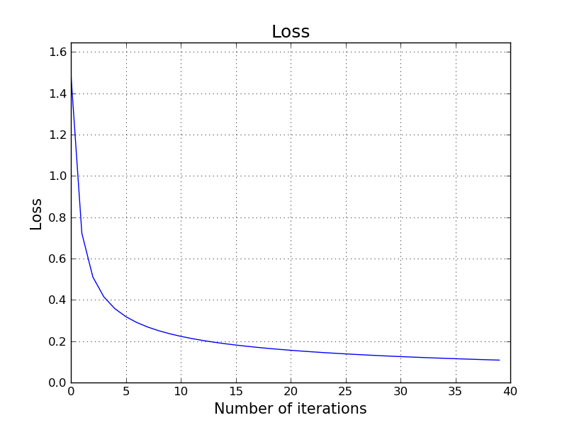
plt.grid()
plt.title('Loss', size=18)
plt.xlabel('Number of iterations', size=15)
plt.ylabel('Loss', size=15)
plt.ylim([0, max(L_cache) * 1.1])
plt.plot(L_cache)

plt.savefig('image.png')

plt.close()
plt.clf()
plt.cla()

Decision Boundary

So, essentially, we have 3 equations:

We have 3 boundaries between all 3 choose 2 of above:

• Equation A - Equation B
• Equation A - Equation C
• Equation B - Equation C

If we plot these three lines:

def plot_decision_boundary(X, Y, W, b, path):
  plt.grid()
  plt.xlim([-2.0, 2.0])
  plt.ylim([-2.0, 2.0])
  plt.xlabel('$x_1$', size=20)
  plt.ylabel('$x_2$', size=20)
  plt.title('Decision boundary', size = 18)

  plt.scatter(X[:, 0], X[:, 1], s=50, c=colormap[y])

  xs = np.array([-2.0, 2.0])
  ys1 = ((b[1, 0] - b[0, 0]) - (W[0, 0] - W[1, 0]) * xs) / (W[0, 1] - W[1, 1])
  ys2 = ((b[2, 0] - b[0, 0]) - (W[0, 0] - W[2, 0]) * xs) / (W[0, 1] - W[2, 1])
  ys3 = ((b[2, 0] - b[1, 0]) - (W[1, 0] - W[2, 0]) * xs) / (W[1, 1] - W[2, 1])

  plt.plot(xs, ys1, c='black')
  plt.plot(xs, ys2, c='black')
  plt.plot(xs, ys3, c='black')

  plt.savefig(path)

plot_decision_boundary(X, Y, W, b, 'image.png')

plt.close()
plt.clf()
plt.cla()

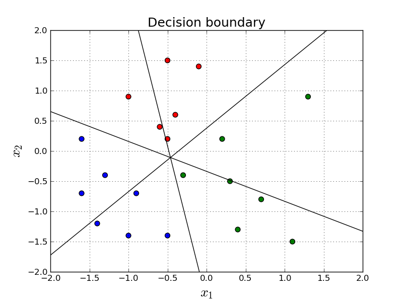
Above, we simply find the boundaries and plot them. The definition of the boundary is the region in which the predictions are equally confident for both of the classifiers. Since we have three classes, there are (3 choose 2) = 3 boundaries.

import matplotlib.animation as animation

fig = plt.figure()

ax = fig.add_subplot(111)
ax.set_xlim([-2.0, 2.0])
ax.set_ylim([-2.0, 2.0])
ax.set_xlabel('$x_1$', size=20)
ax.set_ylabel('$x_2$', size=20)

ax.set_title('Decision boundary - Animated', size = 18)

def animate(i):
  xs = np.array([-2.0, 2.0])
  W = W_cache[i]
  b = b_cache[i]

  ys1 = ((b[1, 0] - b[0, 0]) - (W[0, 0] - W[1, 0]) * xs) / (W[0, 1] - W[1, 1])
  ys2 = ((b[2, 0] - b[0, 0]) - (W[0, 0] - W[2, 0]) * xs) / (W[0, 1] - W[2, 1])
  ys3 = ((b[2, 0] - b[1, 0]) - (W[1, 0] - W[2, 0]) * xs) / (W[1, 1] - W[2, 1])

  lines1.set_data(xs, ys1)
  lines2.set_data(xs, ys2)
  lines3.set_data(xs, ys3)

  text_box.set_text('Iteration: {}'.format(i))
  return lines1, lines2, lines3, text_box

lines1, = ax.plot([], [], c='black')
lines2, = ax.plot([], [], c='black')
lines3, = ax.plot([], [], c='black')

ax.grid()
ax.scatter(X[:, 0], X[:, 1], s=50, c=colormap[y])
text_box = ax.text(1.1, 1.6, 'Iteration 0', size = 16)

anim = animation.FuncAnimation(fig, animate, len(W_cache), blit=False, interval=500)
anim.save('animation.mp4', writer='avconv', fps=6, codec="libx264")

plt.close()
plt.clf()
plt.cla()

As you can see, it starts from a random classifier that does not seem to be working well in the beginning. And the learning process figures out where to go next to find a better classifier. After the learning is done, the final classifier is pretty good, in fact it has 100% accuracy.

Let's see the decision boundary in a more lazy setting. Here, we simply classify every single point in the grid and then give the predictions to some sort of heat map. Comparing to the previous animation, heatmap shows the prediction of every single point in the grid in the final version of the classifiers parameters. On the other hand, the previous animation shows the parameters step by step through the gradient descent iterations.

NX = 100
NY = 100

def plot_decision_boundary_lazy(X, Y, W, b):
  plt.grid()
  plt.xlim([-2.0, 2.0])
  plt.ylim([-2.0, 2.0])
  plt.xlabel('$x_1$', size=20)
  plt.ylabel('$x_2$', size=20)
  plt.title('Decision boundary - Heatmap', size = 18)

  xs = np.linspace(-2.0, 2.0, NX)
  ys = np.linspace(2.0, -2.0, NY)
  xv, yv = np.meshgrid(xs, ys)
  X_fake = np.stack((xv.flatten(), yv.flatten()), axis=1)

  A = []
  for j in range(X_fake.shape[0]):
    x_j = X_fake[j,:].reshape(2,1)
    z_j, a_j = forward_propagate(x_j, W, b)
    A.append(a_j)

  plt.imshow(np.array(A).reshape(NX, NY, 3), extent=[-2.0, 2.0, -2.0, 2.0])
  plt.scatter(X[:, 0], X[:, 1], s=50, c=colormap[y])

  plt.savefig('image.png')

plot_decision_boundary_lazy(X, Y, W_cache[-1], b_cache[-1])

plt.close()
plt.clf()
plt.cla()

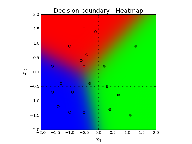
Here, the color of the background depicts our prediction for that imaginary point. Remember that our prediction is $\mathbf{a}$ and it is three dimensional. So, we simply convert that vector to RGB space. So, for example if the prediction is: $[0.98, 0.01, 0.01]$, it will be almost a perfect red, and so on.

If you look closely, you will see some purple color between red and blue points. That is because the predictions in that region is something similar to $[0.45, 0.1, 0.45]$. And this means a mix of red and blue which gives us purple. Similar phenomena happens between other decision boundary intersections.

Here we see the updates of parameters step by step in the gradient descent.

import matplotlib.animation as animation

fig, (ax1, ax2) = plt.subplots(1, 2, figsize=(16, 8), sharex=False, sharey=False)
fig.suptitle('Parameter Updates vs Loss - Animated', size=24)

ax1.grid()
ax1.set_xlim([-0.5, 8.6])
ax1.set_ylim([-5.0, 5.0])
ax1.set_xlabel('Parameter', size=20)
ax1.set_ylabel('Value', size=20)
ax1.set_title('Parameter Values', size = 18)

xlabels = ['$w_{1,1}$', '$w_{1,2}$', '$w_{2,1}$', '$w_{2,2}$',
   '$w_{3,1}$', '$w_{3,2}$', '$b_1$', '$b_2$', '$b_3$']
ax1.set_xticks(range(9))
ax1.set_xticklabels(xlabels, size=20)

ax2.grid()
ax2.set_xlim([0.0, 40])
ax2.set_ylim([0, max(L_cache) * 1.1])
ax2.set_xlabel('Number of iterations', size=20)
ax2.set_ylabel('Loss', size=20)
ax2.set_title('Loss', size=18)

def animate(i):
  ys = np.concatenate((W_cache[i].flatten(), b_cache[i].flatten()))
  xs = np.arange(len(ys))

  for j in range(len(ys)):
    bars[j].set_height(ys[j])

  lines.set_data(range(i+1), L_cache[0:i+1])

  text_box.set_text('Iteration: {}'.format(i))
  return bars, text_box

bars = ax1.bar(range(9), np.zeros(9), color='blue', align='center')
text_box = ax1.text(6.2, 3.6, 'Iteration 0', size = 16)
lines, = ax2.plot([], [], c='black')

anim = animation.FuncAnimation(fig, animate, len(W_cache), blit=False, interval=500)
anim.save('animation.mp4', writer='avconv', fps=4, codec="libx264")

plt.close()
plt.clf()
plt.cla()

This is a nice animation that shows the progress of our parameters $\mathbf{W}$ and $\mathbf{b}$ in each iteration of gradient descent along with the corresponding loss value using the given parameters.

We are starting with small random initial values for: $w_{1,1}, w_{1,2}, w_{2,1}, w_{2,2}, w_{3,1}, w_{3,2}$. We start with all $0$ values for $b_1, b_2, b_3$. Then, we start applying gradient descent. Every step we take in the gradient descent is giving us a better set of parameters so that we see that the loss is decreasing.

Here is how to train the same classifier for the above red, green and blue points using low-level TensorFlow API. It produces exact output with our own hand crafted model. The reason we have the exact output is that we are starting from the same initial $\mathbf{W}$ with our hand-crafted model and also using the same exact learning parameters.

import tensorflow as tf

t_X = tf.placeholder(tf.float32, [None, 2])
t_Y = tf.placeholder(tf.float32, [None, 3])

# t_W = tf.Variable(tf.random_uniform((2, 3)))
t_W = tf.Variable(W_initial.T.astype('f'))
t_b = tf.Variable(tf.zeros((1, 3)))

t_logits = tf.matmul(t_X, t_W) + t_b
t_Softmax = tf.nn.softmax(t_logits)
t_Accuracy = tf.contrib.metrics.accuracy(labels = tf.argmax(t_Y, axis=1),
                                         predictions = tf.argmax(t_Softmax, axis=1))

t_Loss = tf.reduce_mean(tf.nn.softmax_cross_entropy_with_logits(
                         labels=t_Y, logits=t_logits))

train = tf.train.GradientDescentOptimizer(LEARNING_RATE).minimize(t_Loss)
init = tf.global_variables_initializer()

losses = []
accs = []
with tf.Session() as session:
  session.run(init)
  for i in range(NUM_EPOCHS):
    ttrain, loss, acc = session.run([train, t_Loss, t_Accuracy], feed_dict={t_X:X, t_Y:Y})
    losses.append(loss)
    accs.append(acc)

plt.grid()
plt.title('Loss', size=18)
plt.xlabel('Number of iterations', size=15)
plt.ylabel('Loss', size=15)
plt.plot(losses)
plt.ylim([0, max(losses) * 1.1])

plt.savefig('image.png')

plt.close()
plt.clf()
plt.cla()

Exercises

1. If you look at the decision boundary, the three lines of the decision boundary always intersects at one single point. Is this always the case? (i.e., is this an invariant of some sort?) If this is an invariant, why this is the case?
2. Looking to the structure of our decision boundary, try to come up with a set of samples including three classes (red, green and blue) that is linearly separable that our classifier would not be able to successully discriminate all of them.
3. Assume we had four classes: red, green, blue and orange instead of only three classes. How would the decision boundary look like? Try to guess its potential structure. Is that boundary able to classify any linearly separable possible inputs containing four classes?

References

• http://ufldl.stanford.edu/tutorial/supervised/SoftmaxRegression/
• https://eli.thegreenplace.net/2016/the-softmax-function-and-its-derivative/
• http://tutorial.math.lamar.edu/Classes/CalcI/ProductQuotientRule.aspx