Part 3: Building a Simple Neural Network [Draft]
"Truth is ever to be found in the simplicity, and not in the multiplicity and confusion of things." -- Sir Isaac Newton
Introduction
Let's say we want to build a model to discriminate the following red and green points in 2-dimensional space:
import numpy as np
import matplotlib.pyplot as plt
import collections
plt.style.use('classic')
np.set_printoptions(precision=3, suppress=True)

X = np.array([[ 0.65, 0.00],
              [ 0.00,-0.65],
	      [-0.75,-1.29],
	      [ 1.29, 0.75],
	      [-0.46,-0.46],
	      [-1.29,-0.75],
	      [ 0.00, -1.5],
	      [ 0.46, 0.46],
	      [ 0.46,-0.46],
	      [-1.29, 0.75],
 	      [-0.46, 0.46],
	      [ 0.00, 0.65],
	      [ 0.75,-1.29],
	      [ 1.29,-0.75],
	      [-0.65, 0.00],
	      [ 1.50, 0.00],
	      [-1.50, 0.00],
	      [ 0.75, 1.29],
	      [-0.75, 1.29],
	      [ 0.00, 1.50]])
y = np.array([0, 0, 1, 1, 0, 1, 1, 0, 0, 1, 0, 0, 1, 1, 0, 1, 1, 1, 1, 1])

colormap = np.array(['r', 'g'])

def plot_scatter(X, Y, colormap, path):
   plt.grid()
   plt.xlim([-2.0, 2.0])
   plt.ylim([-2.0, 2.0])
   plt.xlabel('$x_1$', size=20)
   plt.ylabel('$x_2$', size=20)
   plt.title('Input 2D points', size=18)
   plt.scatter(X[:,0], X[:,1], s=50, c=colormap[y])
   plt.savefig(path)

plot_scatter(X, y, colormap, 'image.png')

plt.close()
plt.clf()
plt.cla()
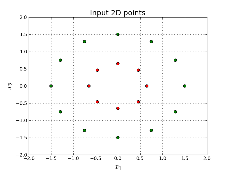
In other words, given a point, $(x_1, x_2)$, we want to output either red, or green. (In this tutorial 0.0 means red and 1.0 means green.)
We can build a simple Neural Network for this problem. Neural Networks are widely used for applications ranging from face recognition, machine translation, speech to text, self driving cars, etc. This is a very simple neural network in terms of number of layers and number of neurons it contains.
It's basically a Logistic Regression (or Softmax Regression) with more layers.
Computation Graph
Here is the visual representation of our model:

and decide if $a^{[3]} > 0.5$ for our final prediction.
Feed-forward Phase
Let's assume that we are given the weights and biases. How do we calculate the output?
We represent $\mathbf{X}$ as a matrix. $\mathbf{X}$ contains all the points. In our case $\mathbf{X}$ contains $m=20$ samples. $\mathbf{y}$ contains all the labels (red or green):
Here is the sizes of the matrices:
- $\mathbf{X}: 20 \times 2$
- $\mathbf{y}: 20 \times 1$
- $\mathbf{W}^{[1]}: 3 \times 2$
- $\mathbf{b}^{[1]}: 3 \times 1$
- $\mathbf{W}^{[2]}: 3 \times 3$
- $\mathbf{b}^{[2]}: 3 \times 1$
- $\mathbf{W}^{[3]}: 1 \times 3$
- $b^{[3]}: 1 \times 1$
Feed-forward basically means given: $\mathbf{x}, y, \mathbf{W}^{[1]}, \mathbf{W}^{[2]}, \mathbf{W}^{[3]}$ and $\mathbf{b}^{[1]}, \mathbf{b}^{[2]}, b^{[3]}$ will produce us $a^{[3]}$. Here is step by step how we do the feed forward phase.
$$ \mathbf{z}^{[1]} = \mathbf{W}^{[1]} \mathbf{x} + \mathbf{b}^{[1]} $$ $$ \mathbf{a}^{[1]} = g(\mathbf{z}^{[1]}) $$ $$ \mathbf{z}^{[2]} = \mathbf{W}^{[2]} \mathbf{a}^{[1]} + \mathbf{b}^{[2]} $$ $$ \mathbf{a}^{[2]} = g(\mathbf{z}^{[2]}) $$ $$ z^{[3]} = \mathbf{W}^{[3]} \mathbf{a}^{[2]} + b^{[3]} $$ $$ a^{[3]} = g(z^{[3]}) $$We are using sigmoid function as the activation $g()$ function as we used before.
Let's try to apply the above equations using an initial random set of weights and bias.
sigmoid = lambda x: 1/(1+np.exp(-x))

def forward_propagate(x, W1, b1, W2, b2, W3, b3):
  z1 = np.matmul(W1, x) + b1
  a1 = sigmoid(z1)

  z2 = np.matmul(W2, a1) + b2
  a2 = sigmoid(z2)

  z3 = np.matmul(W3, a2) + b3
  a3 = sigmoid(z3)

  return z1, a1, z2, a2, z3, a3

W1_initial = np.random.rand(3, 2)
W1 = W1_initial.copy()
b1 = np.zeros((3, 1))
W2_initial = np.random.rand(3, 3)
W2 = W2_initial.copy()
b2 = np.zeros((3, 1))
W3_initial = np.random.rand(1, 3)
W3 = W3_initial.copy()
b3 = np.zeros((1, 1))

z1, a1, z2, a2, z3, a3 = forward_propagate(X[0, :].reshape(2,1), W1, b1, W2, b2, W3, b3)
print(y[0])
print(a3)
0
[[0.802]]
Above we print our prediction for the first point out of 20 points. We use random initial set of weights and bias. We are randomly initializing weights and bias and feed the first $\mathbf{x}$ to our random initial model. As you can see, our prediction is pretty random too, as expected. However, you can see that, given the weights, and bias, it is pretty straight-forward to calculate the final prediction. The tricky part is to learn those weights properly.
Cross Entropy Loss Function
In training, our goal is to learn: $\mathbf{W}^{[1]}, \mathbf{W}^{[2]}, \mathbf{W}^{[3]}, \mathbf{b}^{[1]}, \mathbf{b}^{[2]}, \mathbf{b}^{[3]}$ that best discriminates red and green points. These are called the parameters of our model.
We want to find parameters that minimizes some definition of a cost function. We will use the same cost function we have used before in Logistic Regression and Softmax Regression:
$$ \text{L} = - \sum_{i=1}^{M} y^{(i)} \text{log}( a^{[3](i)} ) + (1 - y^{(i)}) \text{log}( 1 - a^{[3](i)} )$$where $a^{[3](i)}$ is the last layer's activation value corresponding to the $i$ th item in the dataset.
Please see previous lectures if you are interested understanding how we derived the cross entropy loss function.
If we add our loss to our computation graph:

Backpropagation
Now, we are going to have some fun.
Backprop is probably one of the most fundamental algorithms/techniques in Deep Learning. In my opinion, mastering backprop is curicial to be able to (1) fully understand deep learing techniques and (2) to be able to contribute new approaches in the field.
Backpropagation is simply calculating derivatives of loss w.r.t. each parameter in our model. We need this information because we need to feed the derivatives to Gradient Descent. The parameters of the model we want to compute with backprop is:
$$ \frac{d \text{L}}{d \mathbf{W}^{[i]}}, \quad \frac{d \text{L}}{d \mathbf{b}^{[i]}} \quad \forall i \in \{1,2,3\} $$We need to use chain rule, iteratively, to get there. The direction we apply chain rule will be the opposite direction to the feed forward direction. In fact the name backpropagation comes from the fact that we propagate the error (well actually the derivatives, really) through backwards (compared to the feed-forward direction) in a step by step manner.
Here is our updated computation graph after we add the Backprop details.

Recall that we already calculated the first step of derivatives:
$$ \frac{d \text{L}}{dz^{[3]}} = a^{[3]} - y $$in Logistic Regression tutorial. Notice that we are using exactly same loss function. (Both Logistic Regression and the model discussed in this tutorial are a binary classification task.)
Notice that this is defined per sample. So, we have a different $\frac{d \text{L}}{d z^{[3]}}$ value for each sample.
Let's try to go one step further and calculate $\frac{d \text{L}}{d \mathbf{W}^{[3]}}$ by keeping in mind that we already know $\frac{d \text{L}}{dz^{[3]}}$. (This sentence mimicks why we need Chain Rule)
In other words, we know how much $\text{L}$ changes if we play with $z^{[3]}$ and we are trying to find out how much $\text{L}$ changes if we play with $\mathbf{W}^{[3]}$.
Let's look at how we calculate $z^{[3]}$:
$$ \begin{matrix} (\mathbf{W}^{[3]}) \\ \begin{bmatrix} 0 & 0 & 0 \end{bmatrix} \\ \\ \mbox{} \end{matrix} \begin{matrix} (\mathbf{a}^{[2]}) \\ \begin{bmatrix} 0 \\ 0 \\ 0 \\ \end{bmatrix} \end{matrix} + \begin{matrix} (b^{[3]}) \\ \begin{bmatrix} 0 \end{bmatrix} \\ \\ \end{matrix} = \begin{matrix} (z^{[3]}) \\ \begin{bmatrix} 0 \end{bmatrix} \\ \\ \end{matrix} $$Let's look at this equation very carefully. Our simpler task for now is: "How much $z^{[3]}$ will be affected if we play with $\mathbf{W}^{[3]}$?", i.e.,
$$ \frac{d z^{[3]}}{d \mathbf{W}^{[3]}} $$After finding out what the above is, we will extend it and find: $\frac{d \text{L}}{d \mathbf{W}^{[3]}}$ using the Chain Rule.
It seems obvious visually that if we change, say, $\mathbf{W}^{[3](1)}$, $z^{[3]}$ will change proportional to $\mathbf{a}^{[2](1)}$. Notice that we are assuming that $\mathbf{a}^{[2]}$ and $b^{[3]}$ is fixed and frozen. Using similar logic for the other items of $\mathbf{W}^{[3]}$, we can conclude:
$$ \frac{d z^{[3]}}{d \mathbf{W}^{[3]}} = \mathbf{a}^{[2]}.\text{T} $$Similarly, if we change $b^{[3]}$ a small amount, $z^{[3]}$ will also change as same amount in the same direction, so:
$$ \frac{d z^{[3]}}{d b^{[3]}} = 1 $$To finalize the calculation of $\frac{d \text{L}}{d \mathbf{W}^{[3]}}$, for one sample:
$$ \frac{d \text{L}}{d \mathbf{W}^{[3]}} = \frac{d \text{L}}{d z^{[3]}} \frac{d z^{[3]}}{d \mathbf{W}^{[3]}} $$and similarly for $\frac{d \text{L}}{d b^{[3]}}$:
$$ \frac{d \text{L}}{d b^{[3]}} = \frac{d \text{L}}{d z^{[3]}} $$Notice that $\frac{d \text{L}}{dz^{[3]}} \in \mathbb{R}$ and $\frac{dz^{[3]}}{d \mathbf{W}^{[3]}} \in \mathbb{R}^3$. So, it is a scalar multiplication.
Nice.
At this moment, we calculated $\frac{d \text{L}}{d \mathbf{W}^{[3]}}$ and $\frac{d \text{L}}{d b^{[3]}}$. Now, we want to calculate $\frac{d \text{L}}{d \mathbf{W}^{[2]}}$ and $\frac{d \text{L}}{d \mathbf{b}^{[2]}}$. In order to calculate them, we need $\frac{d \text{L}}{d \mathbf{a}^{[2]}}$ and $\frac{d \text{L}}{d \mathbf{z}^{[2]}}$.
Looking to the same figure above visually, and using a similar logic, it looks obvious for one sample:
$$ \frac{d z^{[3]}}{d \mathbf{a}^{[2]}} = \mathbf{W}^{[3]}.\text{T} $$To finalize the calculation of $\frac{d \text{L}}{d \mathbf{a}^{[2]}}$:
$$ \frac{d \text{L}}{d \mathbf{a}^{[2]}} = \frac{d \text{L}}{d z^{[3]}} \frac{d z^{[3]}}{d \mathbf{a}^{[2]}} $$Given $\frac{d \text{L}}{d \mathbf{a}^{[2]}}$, it is easy to get $\frac{d \text{L}}{d \mathbf{z}^{[2]}}$. We just need to apply the gradient of sigmoid function.
$$ \frac{d \text{L}}{d \mathbf{z}^{[2]}} = \frac{d \text{L}}{d \mathbf{a}^{[2]}} \circ \frac{d \mathbf{a}^{[2]}}{d \mathbf{z}^{[2]}} = \frac{d \text{L}}{d \mathbf{a}^{[2]}} \circ \left ( \mathbf{a}^{[2]} \circ \left ( 1 - \mathbf{a}^{[2]} \right ) \right ) $$Now, with knowing $\frac{d \text{L}}{d \mathbf{z}^{[2]}}$, we are set to calculate $\frac{d \text{L}}{d \mathbf{W}^{[2]}}$ and $\frac{d \text{L}}{d \mathbf{b}^{[2]}}$. Here is how we compute $\mathbf{z}^{[2]}$:
$$ \begin{matrix} (\mathbf{W}^{[2]}) \\ \begin{bmatrix} 0 & 0 & 0 \\ 0 & 0 & 0 \\ 0 & 0 & 0 \\ \end{bmatrix} \end{matrix} \begin{matrix} (\mathbf{a}^{[1]}) \\ \begin{bmatrix} 0 \\ 0 \\ 0 \\ \end{bmatrix} \end{matrix} + \begin{matrix} (\mathbf{b}^{[2]}) \\ \begin{bmatrix} 0 \\ 0 \\ 0 \\ \end{bmatrix} \end{matrix} = \begin{matrix} (\mathbf{z}^{[2]}) \\ \begin{bmatrix} 0 \\ 0 \\ 0 \\ \end{bmatrix} \end{matrix} $$It is easy to observe:
$$ \frac{d \mathbf{z}^{[2](1)}}{d \mathbf{W}^{[2]}} = \begin{bmatrix} & \mathbf{a}^{[1]}.T & \\ 0 & 0 & 0 \\ 0 & 0 & 0 \\ \end{bmatrix}, \quad \frac{d \mathbf{z}^{[2](2)}}{d \mathbf{W}^{[2]}} = \begin{bmatrix} 0 & 0 & 0 \\ & \mathbf{a}^{[1]}.T & \\ 0 & 0 & 0 \\ \end{bmatrix}, \quad \frac{d \mathbf{z}^{[2](3)}}{d \mathbf{W}^{[2]}} = \begin{bmatrix} 0 & 0 & 0 \\ 0 & 0 & 0 \\ & \mathbf{a}^{[1]}.T & \\ \end{bmatrix} $$Applying the chain rule, we should do something like:
$$ \frac{d \text{L}}{d \mathbf{W}^{[2]}} = \sum_{i=1}^{3} \frac{d \text{L}}{d \mathbf{z}^{[2](i)}} \frac{d \mathbf{z}^{[2](i)}}{d \mathbf{W}^{[2]}} $$which is a more fancy way of writing:
$$ \frac{d \text{L}}{d \mathbf{W}^{[2]}} = \frac{d \text{L}}{d \mathbf{z}^{[2](1)}} \begin{bmatrix} & \mathbf{a}^{[1]}.T & \\ 0 & 0 & 0 \\ 0 & 0 & 0 \\ \end{bmatrix} + \frac{d \text{L}}{d \mathbf{z}^{[2](2)}} \begin{bmatrix} 0 & 0 & 0 \\ & \mathbf{a}^{[1]}.T & \\ 0 & 0 & 0 \\ \end{bmatrix} + \frac{d \text{L}}{d \mathbf{z}^{[2](3)}} \begin{bmatrix} 0 & 0 & 0 \\ 0 & 0 & 0 \\ & \mathbf{a}^{[1]}.T & \\ \end{bmatrix} $$which is idential to:
$$ \frac{d \text{L}}{d \mathbf{W}^{[2]}} = \begin{bmatrix} \\ \frac{d \text{L}}{d \mathbf{z}^{[2]}} \\ \\ \end{bmatrix} \begin{bmatrix} \mathbf{a}^{[1]}.T \\ \end{bmatrix} $$We are half-way there in terms of finishing the backprop.
We need to calcualte $\frac{d \text{L}}{d \mathbf{a}^{[1]}}$. Let's look at $\frac{d \mathbf{z}^{[2]}}{d \mathbf{a}^{[1]}}$.
$$ \frac{d \text{L}}{\mathbf{a}^{[1](1)}} = \mathbf{W}^{[2](:,1)}.T \frac{d \text{L}}{d \mathbf{z}^{[2]}}, \quad \frac{d \text{L}}{\mathbf{a}^{[1](2)}} = \mathbf{W}^{[2](:,2)}.T \frac{d \text{L}}{d \mathbf{z}^{[2]}}, \quad \frac{d \text{L}}{\mathbf{a}^{[1](3)}} = \mathbf{W}^{[2](:,3)}.T \frac{d \text{L}}{d \mathbf{z}^{[2]}} $$or, equivalently:
$$ \frac{d \text{L}}{\mathbf{a}^{[1]}} = \mathbf{W}^{[2]}.T \frac{d \text{L}}{d \mathbf{z}^{[2]}} $$Now we only missing $\frac{d \text{L}}{d \mathbf{W}^{[1]}}$ and $\frac{d \text{L}}{db^{[1]}}$. Let's look how we calculate $\mathbf{z}^{[1]}$:
$$ \begin{matrix} (\mathbf{W}^{[1]}) \\ \begin{bmatrix} 0 & 0 \\ 0 & 0 \\ 0 & 0 \\ \end{bmatrix} \end{matrix} \begin{matrix} (\mathbf{x}) \\ \begin{bmatrix} 0 \\ 0 \\ \end{bmatrix} \end{matrix} + \begin{matrix} (\mathbf{b}^{[1]}) \\ \begin{bmatrix} 0 \\ 0 \\ 0 \\ \end{bmatrix} \end{matrix} = \begin{matrix} (\mathbf{z}^{[1]}) \\ \begin{bmatrix} 0 \\ 0 \\ 0 \\ \end{bmatrix} \end{matrix} $$Now, let's look at:
$$ \frac{d \text{L}}{d \mathbf{W}^{[1](1,:)}} = \frac{d \text{L}}{d \mathbf{z}^{[1](1)}} \mathbf{x}.\text{T}, \quad \frac{d \text{L}}{d \mathbf{W}^{[1](2,:)}} = \frac{d \text{L}}{d \mathbf{z}^{[1](2)}} \mathbf{x}.\text{T}, \quad \frac{d \text{L}}{d \mathbf{W}^{[1](3,:)}} = \frac{d \text{L}}{d \mathbf{z}^{[1](3)}} \mathbf{x}.\text{T} $$or equivalently:
$$ \frac{d \text{L}}{d \mathbf{W}^{[1]}} = \frac{d \text{L}}{d \mathbf{z}^{[1]}} \mathbf{x}.\text{T} $$and as expected:
$$ \frac{d \text{L}}{d \mathbf{b}^{[1]}} = \frac{d \text{L}}{d \mathbf{z}^{[1]}} $$Let's apply the backprop altogether!
ALPHA = 0.4 # learning rate
def get_loss(y, a):
return -1 * (y * np.log(a) +
(1-y) * np.log(1-a))
def get_loss_numerically_stable(y, z):
return -1 * (y * -1 * np.log(1 + np.exp(-z)) +
(1-y) * (-z - np.log(1 + np.exp(-z))))
def get_gradients_loops(z1, a1, z2, a2, z3, a3, x, y, W1, b1, W2, b2, W3, b3):
dz3 = a3 - y
db3 = dz3
dW3 = dz3 * a2.T
da2 = dz3 * W3.T
dz2 = da2 * (a2 * (1-a2))
db2 = dz2
dW2 = np.matmul(dz2, a1.T)
da1 = np.matmul(W2.T, dz2)
dz1 = da1 * (a1 * (1-a1))
dW1 = np.matmul(dz1, x.T)
db1 = dz1
return dW1, db1, dW2, db2, dW3, db3
def gradient_descent(W1, b1, W2, b2, W3, b3, dW1, db1, dW2, db2, dW3, db3, alpha):
W1 -= alpha * (1.0/20) * dW1
b1 -= alpha * (1.0/20) * db1
W2 -= alpha * (1.0/20) * dW2
b2 -= alpha * (1.0/20) * db2
W3 -= alpha * (1.0/20) * dW3
b3 -= alpha * (1.0/20) * db3
return W1, b1, W2, b2, W3, b3
def get_zero_gradients(W1, b1, W2, b2, W3, b3):
tdW1 = np.zeros_like(W1)
tdb1 = np.zeros_like(b1)
tdW2 = np.zeros_like(W2)
tdb2 = np.zeros_like(b2)
tdW3 = np.zeros_like(W3)
tdb3 = np.zeros_like(b3)
return tdW1, tdb1, tdW2, tdb2, tdW3, tdb3
def add_gradients(tdW1, tdb1, tdW2, tdb2, tdW3, tdb3,
dW1, db1, dW2, db2, dW3, db3):
tdW1 += dW1
tdb1 += db1
tdW2 += dW2
tdb2 += db2
tdW3 += dW3
tdb3 += db3
return tdW1, tdb1, tdW2, tdb2, tdW3, tdb3
L_cache = []
models_cache = []
W1_initial = np.random.rand(3, 2)
W1 = W1_initial.copy()
b1 = np.zeros((3, 1))
W2_initial = np.random.rand(3, 3)
W2 = W2_initial.copy()
b2 = np.zeros((3, 1))
W3_initial = np.random.rand(1, 3)
W3 = W3_initial.copy()
b3 = np.zeros((1, 1))
for i in range(20000):
totalL = 0
tdW1, tdb1, tdW2, tdb2, tdW3, tdb3 = get_zero_gradients(W1, b1, W2, b2, W3, b3)
for j in range(X.shape[0]):
x = X[j, :].reshape(2,1)
z1, a1, z2, a2, z3, a3 = forward_propagate(x, W1, b1, W2, b2, W3, b3)
L = (1.0 / 20) * get_loss_numerically_stable(y[j], z3)
totalL += L
dW1, db1, dW2, db2, dW3, db3 = get_gradients_loops(z1, a1, z2, a2, z3, a3, x, y[j], W1, b1, W2, b2, W3, b3)
tdW1, tdb1, tdW2, tdb2, tdW3, tdb3 = add_gradients(tdW1, tdb1, tdW2, tdb2, tdW3, tdb3,
dW1, db1, dW2, db2, dW3, db3)
W1, b1, W2, b2, W3, b3 = gradient_descent(W1, b1, W2, b2, W3, b3, tdW1, tdb1, tdW2, tdb2, tdW3, tdb3, ALPHA)
models_cache.append((W1.copy(), b1.copy(), W2.copy(), b2.copy(), W3.copy(), b3.copy()))
L_cache.append(totalL[0,0])
if totalL[0,0] < 0.005:
break
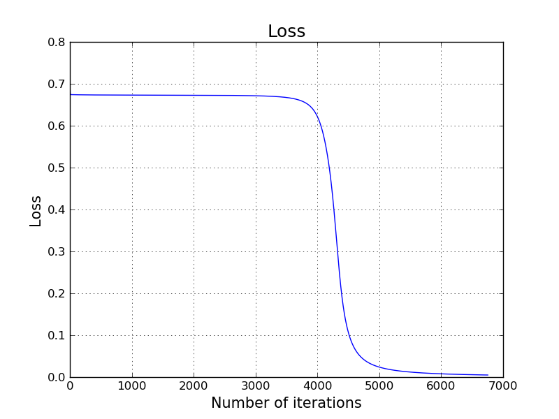
plt.grid()
plt.title('Loss', size=18)
plt.xlabel('Number of iterations', size=15)
plt.ylabel('Loss', size=15)
plt.plot(L_cache)
plt.savefig('image.png')
plt.close()
plt.clf()
plt.cla()
Let's see our inferences on the same points using our classifier.
a3s = []
for j in range(X.shape[0]):
  x = X[j, :].reshape(2,1)
  z1, a1, z2, a2, z3, a3 = forward_propagate(x, W1, b1, W2, b2, W3, b3)
  a3s.append(a3[0,0])

for i,j in zip(y, a3s):
  print(i, j, (j >= 0.5) == (i == 1))
(0, 0.0031506807960418465, True)
(0, 0.006575825913662335, True)
(1, 0.9956909702531819, True)
(1, 0.9968175624933837, True)
(0, 0.004000457461096418, True)
(1, 0.9969317048154863, True)
(1, 0.9970500582174188, True)
(0, 0.011316181722098131, True)
(0, 0.011906281102383126, True)
(1, 0.9966432582082213, True)
(0, 0.0037054959152141888, True)
(0, 0.006797834058656563, True)
(1, 0.9978081334818114, True)
(1, 0.9968844406425068, True)
(0, 0.013487328417851148, True)
(1, 0.9954263746790356, True)
(1, 0.997794064256752, True)
(1, 0.9976105769051488, True)
(1, 0.9956601742298449, True)
(1, 0.9970607102184175, True)
Decision Boundary
Let's try to visualize the decision boundary that error final classifier learns.
The decision boundaries of both Logistic Regression and Softmax Regression were linear. However, the decision boundary of this lecture is not linear, for obvious reasons. Thanks to our non-linear sigmoid function. (Please see Exercise 1)
NX = 40
NY = 40

def plot_decision_boundary_lazy(X, y, W1, b1, W2, b2, W3, b3):
  plt.grid()
  plt.xlim([-2.0, 2.0])
  plt.ylim([-2.0, 2.0])
  plt.xlabel('$x_1$', size=20)
  plt.ylabel('$x_2$', size=20)
  plt.title('Decision boundary - Contour plot', size = 18)

  xs = np.linspace(-2.0, 2.0, NX)
  ys = np.linspace(2.0, -2.0, NY)

  xv, yv = np.meshgrid(xs, ys)

  predictions = []
  for x1, x2 in zip(xv.flatten(), yv.flatten()):
    x = np.array([x1, x2]).reshape(2,1)
    z1, a1, z2, a2, z3, a3 = forward_propagate(x, W1, b1, W2, b2, W3, b3)
    predictions.append(a3)

  predictions = np.array(predictions).reshape(1, NX * NY)
  predictions = np.stack( (1.0 - predictions, predictions, np.zeros((1, NX * NY))) )

  plt.imshow(predictions.T.reshape(NX, NY, 3), extent=[-2.0, 2.0, -2.0, 2.0])
  plt.scatter(X[:,0], X[:,1], s=50, c=colormap[y])

  plt.savefig('image.png')

plot_decision_boundary_lazy(X, y, W1, b1, W2, b2, W3, b3)

plt.close()
plt.clf()
plt.cla()
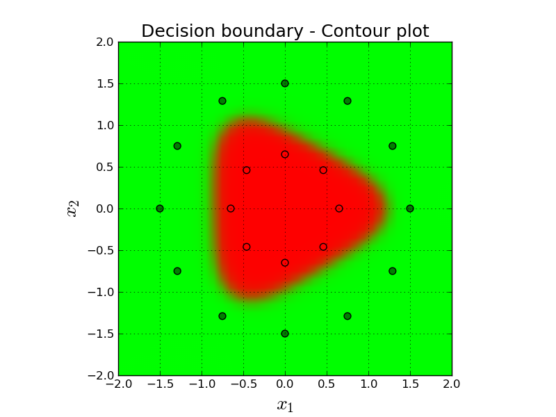
Here, the color of the background depicts our prediction for that imaginary point. Remember that our prediction is one dimensional and between $[0,1]$. If it is $0.0$ it means we are classifying the point confidently as red and if it is $1.0$ we are very confident on green.
In order to create this figure, we simply convert our one dimensional prediction into three dimensions (RGB) using the following logic. R = prediction, G = 1 - prediction, B = 0. So, for example, if our final prediction is, say, 0.9, then the color on that point will be $[0.9, 0.1, 0]$ which is kind of dark green.
Similarly, we can plot the same as our classifier progresses through the learning process. As you may guess, it should start from a random point and get smarter in each step.
import matplotlib.animation as animation

NX = 40
NY = 40

xs = np.linspace(-2.0, 2.0, NX)
ys = np.linspace(2.0, -2.0, NY)
xv, yv = np.meshgrid(xs, ys)

def get_predictions(xv, yv, model):
  predictions = []
  for x1, x2 in zip(xv.flatten(), yv.flatten()):
    x = np.array([x1, x2]).reshape(2,1)
    z1, a1, z2, a2, z3, a3 = forward_propagate(x, *model)
    predictions.append(a3)

  predictions = np.array(predictions).reshape(1, NX * NY)
  predictions = np.stack( (1.0 - predictions, predictions, np.zeros((1, NX * NY))) )
  return predictions.T.reshape(NX, NY, 3)

fig = plt.figure()

ax = fig.add_subplot(111)
ax.set_xlim([-2.0, 2.0])
ax.set_ylim([-2.0, 2.0])
ax.set_xlabel('$x_1$', size=20)
ax.set_ylabel('$x_2$', size=20)

ax.set_title('Decision boundary - Animated', size = 18)

def animate(i):
  im.set_array(get_predictions(xv, yv, models_cache[i * 50]))
  text_box.set_text('Iteration: {}'.format(i * 50))
  return im, text_box

im = ax.imshow(get_predictions(xv, yv, models_cache[0]),
               extent=[-2.0, 2.0, -2.0, 2.0], animated = True)

ax.scatter(X[:,0], X[:,1], s=50, c=colormap[y])
text_box = ax.text(0.6, 1.6, 'Iteration 0', size = 16)

anim = animation.FuncAnimation(fig, animate, len(models_cache) / 50, blit=True, interval=500)
anim.save('animation.mp4', writer='avconv', fps=6, codec="libx264")

plt.close()
plt.clf()
plt.cla()
As you can see, it starts from a random classifier that does not seem to be working well in the beginning. And the learning process figures out where to go next to find a better classifier. After the learning is done, the final classifier is pretty good, in fact it has 100% accuracy.
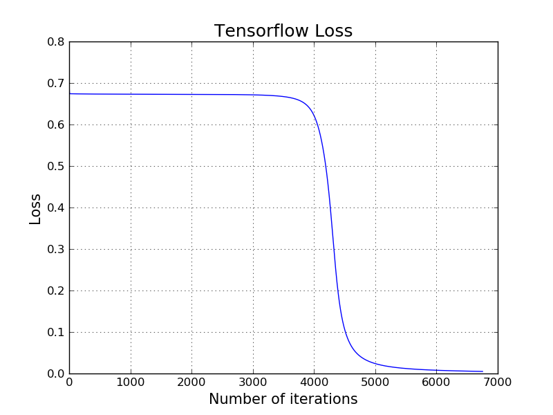
Applying Simple Neural Network using low-level Tensorflow APIs
Here is how to train the same classifier for the above red and green points using low-level TensorFlow API. It produces exact same output with our own hand crafted model. Notice that it is because we start both models from the same initial random starting point (same $W$ and same $b$) using the same learning rate.
import tensorflow as tf

t_X = tf.placeholder(tf.float32, [2, None])
t_Y = tf.placeholder(tf.float32, [1, None])

# t_W1 = tf.Variable(tf.random_uniform((3, 2)))
t_W1 = tf.Variable(W1_initial.astype('f'))
t_b1 = tf.Variable(tf.zeros([3, 1]))

# t_W2 = tf.Variable(tf.random_uniform((3, 3)))
t_W2 = tf.Variable(W2_initial.astype('f'))
t_b2 = tf.Variable(tf.zeros([3, 1]))

#t_W3 = tf.Variable(tf.random_uniform((1, 3)))
t_W3 = tf.Variable(W3_initial.astype('f'))
t_b3 = tf.Variable(tf.zeros([1]))

t_Z1 = tf.matmul(t_W1, t_X) + t_b1
t_A1 = tf.sigmoid(t_Z1)

t_Z2 = tf.matmul(t_W2, t_A1) + t_b2
t_A2 = tf.sigmoid(t_Z2)

t_Z3 = tf.matmul(t_W3, t_A2) + t_b3
t_A3 = tf.sigmoid(t_Z3)

t_Loss = tf.reduce_mean(tf.nn.sigmoid_cross_entropy_with_logits(logits = t_Z3,  labels = t_Y))

train = tf.train.GradientDescentOptimizer(ALPHA).minimize(t_Loss)
init = tf.global_variables_initializer()

with tf.Session() as session:
  session.run(init)
  losses = []
  for i in range(20000):
    ttrain, ttloss = session.run([train, t_Loss], feed_dict={t_X:X.T, t_Y:y.reshape(1,20)})
    losses.append(ttloss)

    if ttloss < 0.005:
      break

plt.grid()
plt.plot(losses)
plt.title('Tensorflow Loss', size = 18)
plt.xlabel('Number of iterations', size=15)
plt.ylabel('Loss', size=15)
plt.savefig('image.png')

plt.close()
plt.clf()
plt.cla()
Exercises
- We claim that the decision boundary of the 3-layer simple neural network as it explained in this chapter is not linear because using a non-linear activation function (sigmoid). However, we have used the same sigmoid function in Logistic Regression as well, and the decision boundary was linear. Also, softmax function doesn't look like linear at all. (Actually, what the heck is the defition (or the test) of a linear function?) And also (assuming sigmoid is a non-linear activation function) why we had a linear decision boundary on logistic regression but not the 3-layer simple neural network?
References
- http://karpathy.github.io/
- http://colah.github.io/
- https://github.com/tensorflow/workshops
- https://cs.nyu.edu/~yann/talks/lecun-20071207-nonconvex.pdf
- https://www.youtube.com/watch?v=8zdo6cnCW2w