Part 1: Logistic Regression [Draft]
"If you can't explain it to a six year old, you don't understand it yourself." -- Albert Einstein
Introduction
Let's say we want to build a model to discriminate the following red and blue points in 2-dimensional space:
import numpy as np
import matplotlib.pyplot as plt
plt.style.use('classic')
np.set_printoptions(precision=3, suppress=True)

X = np.array([[-0.1, 1.4],
              [-0.5,-0.1],
              [ 1.3, 0.9],
              [-0.6, 0.4],
              [-1.5, 0.4],
              [ 0.2, 0.2],
              [-0.3,-0.4],
              [ 0.7,-0.8],
              [ 1.1,-1.5],
              [-1.0, 0.9],
              [-0.5,-1.5],
              [-1.3,-0.4],
              [-1.4,-1.2],
              [-0.9,-1.1],
              [ 0.4,-1.3],
              [-0.4, 0.6],
              [ 0.3,-0.5]])

y = np.array([0, 0, 1, 0, 0, 1, 1, 1, 1, 0, 1, 0, 0, 1, 1, 0, 1])
colormap = np.array(['r', 'b'])

def plot_scatter(X, y, colormap, path):
  plt.grid()
  plt.xlim([-2.0, 2.0])
  plt.ylim([-2.0, 2.0])
  plt.xlabel('$x_1$', size=20)
  plt.ylabel('$x_2$', size=20)
  plt.title('Input 2D points', size=18)
  plt.scatter(X[:,0], X[:, 1], s=50, c=colormap[y])
  plt.savefig(path)

plot_scatter(X, y, colormap, 'image.png')

plt.close()
plt.clf()
plt.cla()
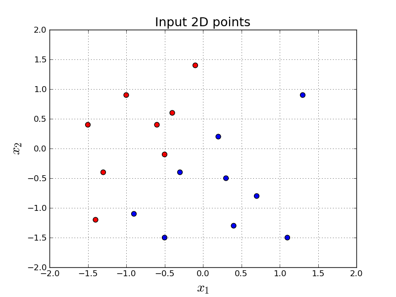
In other words, given a point in 2-dimensions, $\mathbf{x} = (x_1, x_2)$, we want to output either $0$ or $1$. (In this tutorial $0$ represents red, $1$ represents blue.)
We can use Logistic Regression for this problem. In Logistic Regression, we first learn weights, $\mathbf{w} = (w_1, w_2)$, and bias, $b$. This phase of learning these weights and the bias is called training. Then we use the following formula to predict if the new point is red or blue. This phase is called prediction or inference.
In this tutorial, we will use the following equation to predict the class of a new point:
\begin{equation} \label{eq:sigmoid_eq} a = \frac{1}{1+e^{-(w_1x_1 + w_2x_2 + b)}} \end{equation}
In the above equation, we can see that $0 < a < 1$. This is a useful property of the sigmoid function. We will see what sigmoid function is in a second.
Let's see how we are going to finalize our prediction (our guess) for a given point $\mathbf{x}$:
\begin{equation} \label{eq:inference} \text{Our prediction} = \begin{cases} 0, & \text{if}\ \quad a < 0.5 \\ 1, & \text{otherwise} \end{cases} \end{equation}
The parameters of the Logistic Regression model are: weights, $\mathbf{w} = (w_1, w_2)$ and bias, $b$. These parameters are learned with a learning algorithm. After they are learned, we apply them using the above procedure to predict the class of a new sample.
Let's make an example prediction for a new given point. Let's assume somebody already learned some weights, $\mathbf{w}$, and bias, $b$ for us:
$$ \mathbf{w} = \begin{bmatrix} 6.33 & -4.22 \end{bmatrix}, \quad b=1.99 $$For a new given point, $\mathbf{x} = (x_1, x_2)$, in the two dimensional space, say, $\mathbf{x} = \begin{bmatrix} 1.1 & -0.6 \end{bmatrix}$, we can predict the class using Equation \ref{eq:sigmoid_eq} and \ref{eq:inference}.
sigmoid = lambda x: 1/(1+np.exp(-x))

w = np.array([6.33, -4.22])   # some magical w
b = 1.99                      # some magical b
x = np.array([1.1, -0.6])     # point we want to classify

print(sigmoid(w.dot(x) + b))
0.9999897169153853
Let's try another point, $\mathbf{x} = \begin{bmatrix} -1.2 & 1.0 \end{bmatrix}$.
sigmoid = lambda x: 1/(1+np.exp(-x))

w = np.array([6.33, -4.22])   # some magical w
b = 1.99                      # some magical b
x = np.array([-1.2, 1.0])     # point we want to classify

print(sigmoid(w.dot(x) + b))
5.402552018717133e-05
We see that we get a value close to $1$ first and close to $0$ secondly. Remember: if the value is smaller than 0.5, it means our prediction is red and otherwise it is blue.
Computation Graph
Here is a visual representation of our model:

or alternatively we can visualize the same:

We typically see the first version of the computation graph visualization more than the second one in the literature. The first version looks more compact. However, I personally enjoy the second one better since it is more explicit in terms of the input-output at each node.
In the second representation, if there is an arrow from node $A$ to node $B$, it means $A$ is needed to compute $B$. It is that simple. We will dive more into computation graph internals in the following tutorials.
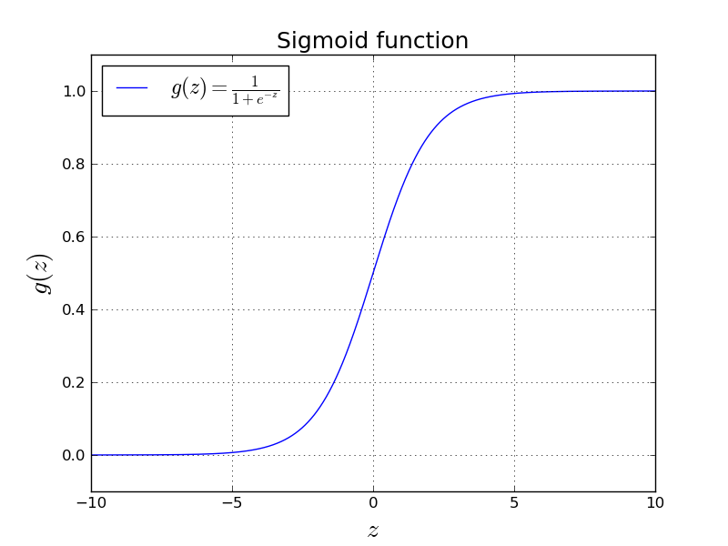
We use sigmoid function as $g(z)$ in logistic regression:
$$ g(z) = \frac{1}{1+e^{-z}} $$We can intuitively see that $0 < g(z) < 1$ for any given $z \in \mathbb{R}$. Here is how $g(z)$ behaves in some useful range.
sigmoid = lambda x: 1/(1+np.exp(-x))

def plot_sigmoid():
  plt.grid()
  plt.xlim([-10.0, 10.0])
  plt.ylim([-0.1, 1.1])
  xs = np.arange(-10, 10, 0.001)
  plt.xlabel('$z$', size=20)
  plt.ylabel('$g(z)$', size=20)
  plt.title('Sigmoid function', size=18)
  plt.plot(xs, sigmoid(xs), label=r'$g(z)= \frac{1}{1+e^{-z}}$')
  plt.legend(loc='upper left', fontsize=17)
  plt.savefig('image.png')

plot_sigmoid()

plt.close()
plt.clf()
plt.cla()
Maximum Likelihood Estimation
In training, our goal is to learn three numbers: $w_1, w_2, b$ that best discriminates red and blue points.
We want to find $w_1, w_2, b$ that minimizes some definition of a cost function. Let's attempt to write a cost function for this problem.
Let's say we have two points:
$$\mathbf{x}^{(1)} = \begin{bmatrix} -0.1 & 1.4 \end{bmatrix}, \quad y^{(1)} = 0$$and similarly:
$$\mathbf{x}^{(2)} = \begin{bmatrix} 1.3 & 0.9 \end{bmatrix}, \quad y^{(2)} = 1$$We want a classifier that produces very high $a$ when $y=1$, and conversely very low $a$ when $y=0$. We hope that $a$ is very close to $y$ for each sample.
In other words,
- If $y=1$, we want to maximize $a$.
- If $y=0$, we want to maximize $1-a$.
If we combine (1) and (2), we want to maximize:
$$a^y.(1-a)^{(1-y)}$$Maximizing above is equal to maximizing:
$$ \text{log}(a^y.(1-a)^{(1-y)}) = y\text{log}(a) + (1-y) \text{log}(1-a) $$or we want to minimize:
$$ \text{L} = -(y\text{log}(a) + (1-y) \text{log}(1-a)) $$Generally, in Machine Learning we like to minimize the loss. That is why we changed the direction. This is by convention. We call the above $\text{L}$, which stands for loss.
The above formula defines a cost function (or loss) for only one sample. We also need a loss function for multiple samples (which we will call $\text{J}$).
Let's start by an example. Say, we have three positive samples and two different classifiers. Here is the $a$ values for those three samples for each of the classifier:
- Classifier 1: 0.9, 0.4, 0.8
- Classifier 2: 0.7, 0.7, 0.7
There are multiple answers for this question. One of the answers is Maximum Likelihood Estimation (MLE). MLE decides this question by multiplying those numbers and taking the maximum:
- Classifier 1: $0.9 \times 0.4 \times 0.8 \simeq 0.29$
- Classifier 2: $0.7 \times 0.7 \times 0.7 \simeq 0.34$
this is called maximum likelihood. Maximizing the above is equal to maximizing below:
$$ \begin{align*} & = \text{log} \left( \prod_{i=1}^{m} a^{(i)^{y^{(i)}}} . (1-a^{(i)})^{(1-y^{(i)})} \right ) \\ & = \sum_{i=1}^m \text{log} \left( a^{(i)^{y^{(i)}}} . (1-a^{(i)})^{(1-y^{(i)})} \right ) \\ & = \sum_{i=1}^m {y^{(i)}} \text{log} \left( a^{(i)} \right ) + (1-y^{(i)}) \text{log} \left ( 1-a^{(i)} \right ) \end{align*} $$or, equivalently, we need to minimize:
$$ \text{J} = - \sum_{i=1}^m {y^{(i)}} \text{log} \left( a^{(i)} \right ) + (1-y^{(i)}) \text{log} \left ( 1-a^{(i)} \right ) $$Here we use the notation $\text{J}$ for the quantity we want to minimize for all samples, and $\text{L}$ for one sample. Let's add these to our computation graph visualization:

We kept the computation graph simpler by only showing the Loss for one sample.
Gradient Descent
Gradient descent is probably one of the most beautiful algorithm ever invented. It is an iterative algorithm that makes the output better and better in each step. In each iteration, we make a step towards to the opposite of the gradient. Hence, it is gradient descent.
Let's think about how we would minimize $f(x) = x^2 + 6x + 5$, numerically:
f = lambda x: x**2 + 6*x + 5

def plot_func():
  plt.grid()
  xs = np.arange(-10, 10, 0.001)
  plt.xlim([-10, 10])
  plt.xlabel('$x$', size=20)
  plt.ylabel('$f(x)$', size=20)
  plt.title('Some arbitrary function', size=18)
  plt.plot(xs, f(xs), label=r'$f(x)= x^2 + 6x + 5$')
  plt.scatter([6], [f(6)], c='red', s=50)
  plt.legend(loc='upper left', fontsize=17)
  plt.savefig('image.png')

plot_func()

plt.close()
plt.clf()
plt.cla()
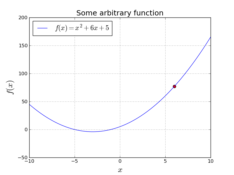
Let's say we started with $x=6$ and we want to take step that will make $f(x)$ smaller.
We have two questions to ask here:
- Should we walk to the left or to the right?
- How much should we walk?
In gradient descent, we decide those by looking to the:
$$ \frac{df}{dx} = 2x + 6 $$This is the slope of $f(x)$ at each $x$. So, if slope is positive, we want to go to left, and if slope is negative, we want to go to right. (Assuming we want to minimize.)
Intuitively, we want to take a big step if the slope is big, and a smaller step if slope is relatively small. However, we may want to play with the size of our steps, so we invent a new parameter: learning rate . We will use $\alpha$ to denote learning rate.
import matplotlib.animation as animation

f = lambda x: x**2 + 6*x + 5
x = 6.0
LEARNING_RATE = 0.1

steps = []
for i in range(21):
  steps.append([x, f(x)])
  x = x - LEARNING_RATE * (2 * x + 6)

steps = np.array(steps)

def animate(i):
  scatter_points.set_offsets(steps[0:i+1,:])
  text_box.set_text('Iteration: {}'.format(i))

  return scatter_points, text_box

fig = plt.figure()
xs = np.arange(-10, 10, 0.001)
ax = fig.add_subplot(111)
ax.set_title('Gradient descent updates', size=18)
ax.set_xlim([-10.0, 10.0])
ax.set_xlabel('$x$', size=20)
ax.set_ylabel('$f(x)$', size=20)
ax.grid()
ax.plot(xs, f(xs), label=r'$f(x)= x^2 + 6x + 5$')
ax.legend(loc='upper left', fontsize=17)

scatter_points = ax.scatter([], [], c='red', s=50)
text_box = ax.text(4, 170, '', size = 16)

anim = animation.FuncAnimation(fig, animate, 20, blit=True, interval=500)
anim.save('animation.mp4', writer='avconv', fps=2, codec="libx264")

plt.close()
plt.clf()
plt.cla()
What if we had a more complex surface? Maybe two dimensional? For example:
from mpl_toolkits.mplot3d.axes3d import Axes3D

f = lambda x,y: x**2 + y**2

NX = 100
NY = 100

xs = np.linspace(-4, 4, NX)
ys = np.linspace(-4, 4, NY)
xv, yv = np.meshgrid(xs, ys)

zv = f(yv.flatten(), xv.flatten())

plt.grid()
fig = plt.figure()
fig.suptitle('Some arbitrary function: $f(x_1,x_2) = x_1^2 + x_2^2$', fontsize=15)
ax = fig.add_subplot(1, 1, 1, projection='3d')
ax.set_xlabel('$x_1$', size=16)
ax.set_ylabel('$x_2$', size=16)
ax.plot_surface(xv, yv, zv.reshape(NX, NY), rstride=4, cstride=4, alpha=0.25)
ax.scatter([-3.2], [-3.2], [f(-3.2, -3.2)], c='red', s=50)
ax.view_init(55, 35)

plt.xlim([-4, 4])
plt.ylim([-4, 4])

fig.tight_layout()
plt.savefig('image.png')

plt.close()
plt.clf()
plt.cla()
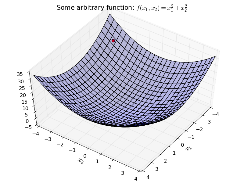
We can apply the same idea here as well.
Start with a random initial point. For each direction $x_1$ and $x_2$, independently go in the opposite direction of the derivative.
f = lambda x,y: x**2 + y**2
NX = 100
NY = 100

x1 = -3.2
x2 = -3.2
LEARNING_RATE = 0.1

steps = []
for i in range(21):
  steps.append([x1, x2])
  x1 = x1 - LEARNING_RATE * (2 * x1)
  x2 = x2 - LEARNING_RATE * (2 * x2)

steps = np.array(steps)

xs = np.linspace(-4, 4, NX)
ys = np.linspace(-4, 4, NY)
xv, yv = np.meshgrid(xs, ys)

zv = f(yv.flatten(), xv.flatten())

plt.grid()
fig = plt.figure()
fig.suptitle('Some arbitrary function: $f(x_1,x_2) = x_1^2 + x_2^2$', fontsize=15)
ax = fig.add_subplot(1, 1, 1, projection='3d')
ax.set_xlabel('$x_1$', size=16)
ax.set_ylabel('$x_2$', size=16)
ax.plot_surface(xv, yv, zv.reshape(NX, NY), rstride=4, cstride=4, alpha=0.25)
ax.view_init(55, 35)

plt.xlim([-4, 4])
plt.ylim([-4, 4])

fig.tight_layout()

def animate(i):
  graph.set_offsets(steps[i,:])
  graph.set_3d_properties([f(*steps[i,:])], zdir='z')
  text_box.set_text('Iteration: {}'.format(i))
  return graph, text_box

graph = ax.scatter([], [], [], s=50, c='red')
lines, = ax.plot([], [], [], c='red')

text_box = ax.text(-4, 3, 500.0, 'Iteration 0', size = 16)

anim = animation.FuncAnimation(fig, animate, 20, interval=50, blit=True)
anim.save('animation.mp4', writer='avconv', fps=2, codec="libx264")

plt.close()
plt.clf()
plt.cla()
We simply applied this gradient descent rule:
$$ \begin{align*} x_1 &= x_1 - \alpha \frac{\partial f}{\partial x_1} \\ x_2 &= x_2 - \alpha \frac{\partial f}{\partial x_2} \\ \end{align*} $$where $\alpha$ is the learning parameter.
We will apply exactly the same idea in Logistic Regression as well.
In order to do gradient descent, we need the derivatives:
$$ \frac{\partial \text{L}}{\partial w_1}, \quad \frac{\partial \text{L}}{\partial w_2}, \quad \frac{\partial \text{L}}{\partial b} $$We need to do some calculus to calculate the derivatives. We will apply the chain rule.
Chain Rule
Let's look at our computation graph again.
Here is the application of the Chain Rule for our case:
$$ \frac{\partial \text{L}}{\partial w_1} = \frac{\partial \text{L}}{\partial a} \frac{d a}{d z} \frac{\partial z}{\partial w_1}, \quad \frac{\partial \text{L}}{\partial w_2} = \frac{\partial \text{L}}{\partial a} \frac{d a}{d z} \frac{\partial z}{\partial w_2}, \quad \frac{\partial \text{L}}{\partial b} = \frac{\partial \text{L}}{\partial a} \frac{d a}{d z} \frac{\partial z}{\partial b} $$After really understanding the above equation, the rest is simple mathematics.
Let's do some calculus.


Now, let's combine the above three equations.
$$ \begin{align*} \frac{\partial L}{\partial z} &= \frac{\partial \text{L}}{\partial a} \frac{d a}{d z} = \left ( \frac{-y}{a} + \frac{1-y}{1-a} \right ) \left ( a (1-a) \right ) \\ & = \frac{-y}{a} a (1-a) + \frac{1-y}{1-a} a(1-a) = -y (1-a) + (1-y) a = -y + ya + a - ya = a - y \end{align*} $$And finally, our final step:
$$ \frac{\partial \text{L}}{\partial w_1} = \frac{\partial \text{L}}{d z} \frac{\partial z}{\partial w_1} = (a - y) x_1, \quad \frac{\partial \text{L}}{\partial w_2} = \frac{\partial \text{L}}{\partial z} \frac{\partial z}{\partial w_2} = (a - y) x_2, \quad \frac{\partial \text{L}}{\partial b} = \frac{\partial \text{L}}{\partial z} \frac{\partial z}{\partial b} = (a - y) $$We took the derivative of sigmoid function while deriving the above gradients:
$$ \frac{d a}{d z} = g(z) (1-g(z)) $$Let's see how this actually looks like:
sigmoid_der = lambda x: sigmoid(x)*(1-sigmoid(x))

def plot_sigmoid_der():
   plt.grid()
   plt.xlim([-10.0, 10.0])
   plt.ylim([-0.1, 0.4])
   xs = np.arange(-10, 10, 0.001)
   plt.xlabel('$z$', size=20)
   plt.ylabel("$g'(z)$", size=20)
   plt.title('Derivative of sigmoid function', size=18)
   plt.plot(xs, sigmoid_der(xs), label=r"$g'(z) = g(z)(1-g(z))}}$")
   plt.legend(loc='upper left', fontsize=17)
   plt.savefig('image.png')

plot_sigmoid_der()

plt.close()
plt.clf()
plt.cla()
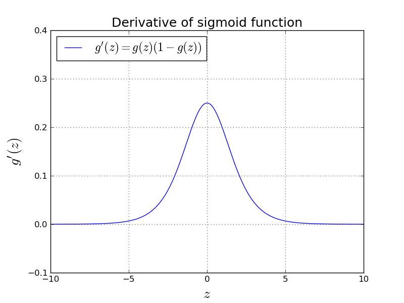
This intuitively means that the change close to $0$ is fast, but when you get far
away than $0$ the change gets slower.
Numerical Stability of the Loss function
There is only one thing remaining before we can start coding.
Here is the loss function we came up with:
$$ \text{L} = -(y\text{log}(a) + (1-y) \text{log}(1-a)) $$Notice that $y \in \{0,1\}$ and $0 < a < 1$. What are the possible values for $\text{L}$? Let's look at the natural logarithm function.
def plot_natural_log():
   plt.grid()
   plt.xlim([-0.5, 8.0])
   xs = np.arange(0.000000001, 8.0, 0.0001)
   plt.xlabel('$x$', size=20)
   plt.ylabel("$log(x)$", size=20)
   plt.title('Natural log function.', size=18)
   plt.plot(xs, np.log(xs), label=r"$log(x)$")
   plt.legend(loc='upper left', fontsize=17)
   plt.savefig('image.png')

plot_natural_log()

plt.close()
plt.clf()
plt.cla()
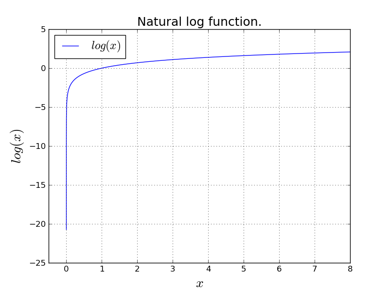
An important observation is that $\text{log}(0)$ approaches to $- \infty$. This is numerically an issue.
Not only that, more importantly, $\text{log}(x)$ becomes unstable for small values of $x$. This means a small change in $x$ because of floating point representation issues, will play a big role in $\text{log}(x)$ which will give the algorithm unstable nature. (harder to converge, etc.)
So, we will try to: come up with mathematically equal way that is numerically okay.
Let's see what we can do. We know that:
$$ \text{L} = -(y\text{log}(a) + (1-y) \text{log}(1-a)) $$and also we know:
$$ a = \frac{1}{1+e^{-z}} $$Let's try to compute $\text{L}$ without explicitly computing $\text{log}(a)$.
Plugging $a$ into $\text{L}$:
$$ \begin{align*} \text{L} & = - \left ( y\text{log} \left (\frac{1}{1+e^{-z}} \right ) + (1-y) \text{log} \left (1-\frac{1}{1+e^{-z}}\right) \right) \\ & = - \left ( y\text{log} \left (\frac{1}{1+e^{-z}} \right ) + (1-y) \text{log} \left (\frac{e^{-z}}{1+e^{-z}}\right) \right) \\ & = - \left ( - y \text{log} \left ( 1+e^{-z} \right ) + (1-y) \left ( \text{log} (e^{-z}) - \text{log} (1 + e^{-z}) \right ) \right ) \\ & = - \left ( - y \text{log} \left ( 1+e^{-z} \right ) + (1-y) \left ( -z - \text{log} (1 + e^{-z}) \right ) \right ) \end{align*} $$And we are done.
This is numerically stable because every time we are calling $\text{log}$, it is not in the critical unstable range.
Applying Gradient Descent
LEARNING_RATE = 8.0
NUM_EPOCHS = 20

def get_loss(y, a):
  return -1 * (y * np.log(a) +
               (1-y) * np.log(1-a))

def get_loss_numerically_stable(y, z):
   return -1 * (y * -1 * np.log(1 + np.exp(-z)) +
                (1-y) * (-z - np.log(1 + np.exp(-z))))

w_cache = []
b_cache = []
l_cache = []

# some nice initial value, so that the plot looks nice.
w = np.array([-4.0, 29.0])
b = 0.0

for i in range(NUM_EPOCHS):
  dw = np.zeros(w.shape)
  db = 0.0
  loss = 0.0

  for j in range(X.shape[0]):
    x_j = X[j,:]
    y_j = y[j]

    z_j = w.dot(x_j) + b
    a_j = sigmoid(z_j)

    loss_j = get_loss_numerically_stable(y_j, z_j)

    dw_j = x_j * (a_j-y_j)
    db_j = a_j - y_j

    dw += dw_j
    db += db_j
    loss += loss_j

  # because we have 17 samples
  dw = (1.0/17) * dw
  db = (1.0/17) * db
  loss = (1.0/17) * loss

  w -= LEARNING_RATE * dw
  b -= LEARNING_RATE * db

  w_cache.append(w.copy())
  b_cache.append(b)
  l_cache.append(loss)

plt.grid()
plt.title('Loss', size=18)
plt.xlabel('Number of iterations', size=15)
plt.ylabel('Loss', size=15)
plt.plot(l_cache)

plt.savefig('image.png')

plt.close()
plt.clf()
plt.cla()
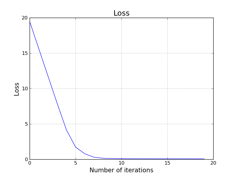
It turns out we just trained a pretty good classifier for this problem. We achieved 100% accuracy. Let's try to visualize our decision boundary.
Remember: if the value is smaller than 0.5, it means our prediction is red and otherwise it is blue. (see Equation \ref{eq:inference})Decision Boundary
We predict red if:
$$ \frac{1}{1+e^{-(w_1x_1+w_2x_2+b)}} < 0.5 $$and blue otherwise.
So, our decision boundary is:
$$ \frac{1}{1+e^{-(w_1x_1+w_2x_2+b)}} = 0.5 $$If we do some math:
$$ e^{-(w_1x_1+w_2x_2+b)} = 1 $$ $$ w_1x_1+w_2x_2+b = 0 $$ $$ x_2 = \frac{-w_1x_1 - b}{w_2} $$Now, let's see what will be the value of $x_2$ when $x_1=-1.5$ and $x_1 =1.5$.
def plot_decision_boundary(X, y, w, b, path):
   plt.grid()
   plt.xlim([-2.0, 2.0])
   plt.ylim([-2.0, 2.0])
   plt.xlabel('$x_1$', size=20)
   plt.ylabel('$x_2$', size=20)
   plt.title('Decision boundary', size = 18)

   xs = np.array([-2.0, 2.0])
   ys = (-w[0] * xs - b)/w[1]

   plt.scatter(X[:,0], X[:,1], s=50, c=colormap[y])
   plt.plot(xs, ys, c='black')
   plt.savefig(path)

plot_decision_boundary(X, y, w_cache[-1], b_cache[-1], 'image.png')

plt.close()
plt.clf()
plt.cla()
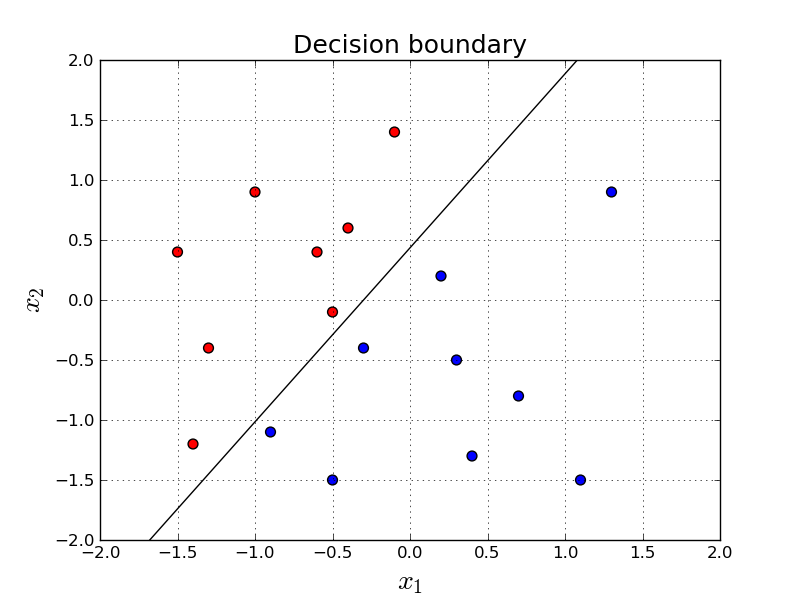
Nice. How do we know we have a linear classifier?
We can do better. Now, let's see the decision boundary step by step as an animation. Everybody loves animations.
import matplotlib.animation as animation

fig = plt.figure()

ax = fig.add_subplot(111)
ax.set_xlim([-2.0, 2.0])
ax.set_ylim([-2.0, 2.0])
ax.set_xlabel('$x_1$', size=20)
ax.set_ylabel('$x_2$', size=20)

ax.set_title('Decision boundary - Animated', size = 18)

def animate(i):
  xs = np.array([-2.0, 2.0])
  ys = (-w_cache[i][0] * xs - b)/w_cache[i][1]
  lines.set_data(xs, ys)

  text_box.set_text('Iteration: {}'.format(i))

  return lines, text_box

lines, = ax.plot([], [], c='black')
ax.scatter(X[:,0], X[:,1], s=50, c=colormap[y])
text_box = ax.text(1.1, 1.6, 'Iteration 0', size = 16)

anim = animation.FuncAnimation(fig, animate, len(w_cache), blit=True, interval=500)
anim.save('animation.mp4', writer='avconv', fps=2, codec="libx264")

plt.close()
plt.clf()
plt.cla()
Let's see the decision boundary in a more lazy setting. Here, we simply classify every single point in the grid and then give the predictions to a contour plot. Comparing to the previous animation, contour plot shows the prediction of every single point in the grid in the final version of the classifiers parameters. On the other hand, the previous animation shows the parameters step by step through the gradient descent iterations.
NX = 100
NY = 100

def plot_decision_boundary_lazy(X, y, w, b):
  plt.grid()
  plt.xlim([-2.0, 2.0])
  plt.ylim([-2.0, 2.0])
  plt.xlabel('$x_1$', size=20)
  plt.ylabel('$x_2$', size=20)
  plt.title('Decision boundary - Lazy setting', size = 18)

  xs = np.linspace(-2.0, 2.0, NX)
  ys = np.linspace(2.0, -2.0, NY)
  xv, yv = np.meshgrid(xs, ys)

  X_fake = np.stack((xv.flatten(), yv.flatten()), axis=1)

  predictions = []
  for i in range(X_fake.shape[0]):
    predictions.append(sigmoid(w.dot(X_fake[i,:]) + b))

  predictions = np.array(predictions)
  predictions = np.stack( (1-predictions, np.zeros(NX * NY), predictions) )
  plt.imshow(predictions.T.reshape(NX, NY, 3), extent=[-2.0, 2.0, -2.0, 2.0])
  plt.scatter(X[:, 0], X[:, 1], s=50, c=colormap[y])

  plt.savefig('image.png')

plot_decision_boundary_lazy(X, y, w_cache[-1], b_cache[-1])

plt.close()
plt.clf()
plt.cla()
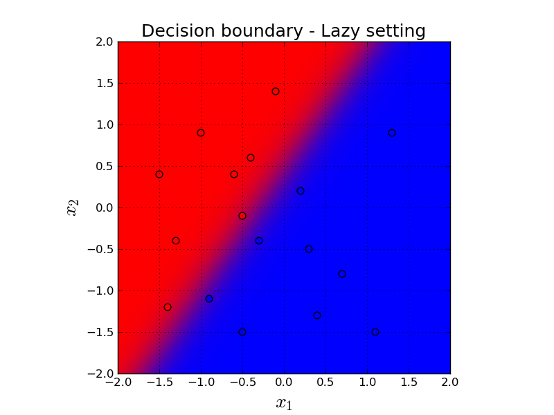
Here, background red means our prediction is very close to $0$ which means it is confidently classified as red. And conversely, background blue means our prediction is very close to $1$ which means it is confidently classified as blue.
For our predictions in the purpleish middle area, we are not confident on our predictions. Our predictions are close to $0.5$, as expected.
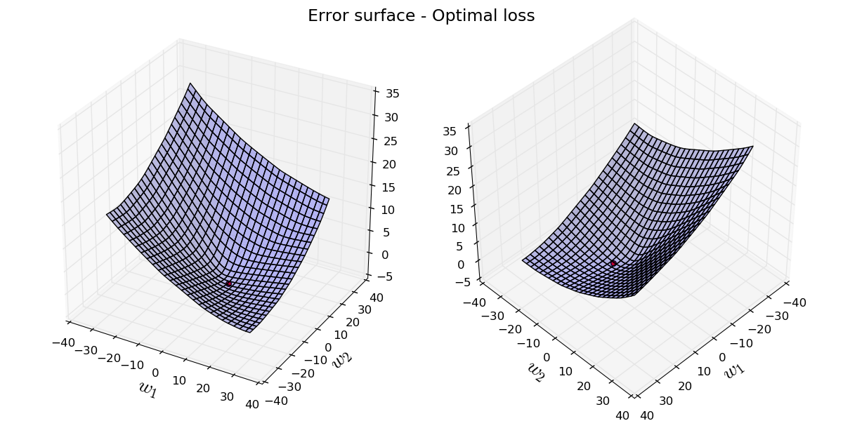
Visualizing the Error Surface
We can also visualize the loss as a function of $\mathbf{w}$, on 2-D surface. Here, we fix $b$ to the optimal value, and plug all possible values of $\mathbf{w}$ and compute the error value for that given $\mathbf{w}$ with that fixed $b$. This surface has an interesting property of being convex.
from mpl_toolkits.mplot3d.axes3d import Axes3D

NX = 100
NY = 100

def get_average_loss(X, w, b):
  total_loss = 0.0
  for i in range(X.shape[0]):
    x_i = X[i,:]
    z = w.dot(x_i) + b
    total_loss += get_loss_numerically_stable(y[i], z)
  return total_loss / X.shape[0]

xs = np.linspace(-30, 30, NX)
ys = np.linspace(-30, 30, NY)
xv, yv = np.meshgrid(xs, ys)

w_fake = np.stack((xv.flatten(), yv.flatten()), axis=1)

losses = []
for i in range(w_fake.shape[0]):
  losses.append( get_average_loss(X, w_fake[i,:], b_cache[-1]) )

losses = np.array(losses)
min_loss = np.min(losses)

def plot_error_surface(X, y, best_w):
  plt.grid()

  fig = plt.figure(figsize=(12,6))
  fig.suptitle('Error surface - Optimal loss', fontsize=17)
  ax = fig.add_subplot(1, 2, 1, projection='3d')
  ax.set_xlabel('$w_1$', size=20)
  ax.set_ylabel('$w_2$', size=20)
  ax.plot_surface(xv, yv, losses.reshape(NX, NY), rstride=4, cstride=4, alpha=0.25)
  ax.scatter(best_w[0], best_w[1], [min_loss], s=30, c='red')

  ax = fig.add_subplot(1, 2, 2, projection='3d')
  ax.set_xlabel('$w_1$', size=20)
  ax.set_ylabel('$w_2$', size=20)
  ax.plot_surface(xv, yv, losses.reshape(NX, NY), rstride=4, cstride=4, alpha=0.25)
  ax.scatter(best_w[0], best_w[1], [min_loss], s=30, c='red')
  ax.view_init(45, 45)

  fig.tight_layout()
  plt.savefig('image.png')

plot_error_surface(X, y, w_cache[-1])

plt.close()
plt.clf()
plt.cla()
Let's see the parameters step by step through the iterations of gradient descent. We start from a random initial point and keep iterating to refine our parameters.
NX = 100
NY = 100

fig = plt.figure(figsize=(12,6))
ax = fig.add_subplot(111, projection='3d')
ax.set_xlim3d([-40, 40.0])
ax.set_ylim3d([-40, 40.0])
ax.set_xlabel('$w_1$', size=20)
ax.set_ylabel('$w_2$', size=20)

ax.set_title('Gradient descent updates', fontsize=17)
ax.plot_surface(xv, yv, losses.reshape(NX, NY), rstride=4, cstride=4, alpha=0.25)

def animate(i):
  graph.set_offsets([w_cache[i][0], w_cache[i][1]])
  graph.set_3d_properties([l_cache[i]], zdir='z')

  line_data[0].append(w_cache[i].flatten()[0])
  line_data[1].append(w_cache[i].flatten()[1])
  line_data[2].append(l_cache[i])

  lines.set_data(line_data[0], line_data[1])
  lines.set_3d_properties(line_data[2])

  text_box.set_text('Iteration: {}'.format(i))

  return graph, lines, text_box

line_data = [[], [], []]
graph = ax.scatter([], [], [], s=50, c='red')
lines, = ax.plot([], [], [], c='red')

text_box = ax.text(20.0, 20.0, 500.0, 'Iteration 0', size = 16)

anim = animation.FuncAnimation(fig, animate, len(w_cache), interval=50, blit=True)
anim.save('animation.mp4', writer='avconv', fps=2, codec="libx264")

plt.close()
plt.clf()
plt.cla()
Applying Logistic Regression using low-level Tensorflow APIs
TensorFlow is an open-source software library for Machine Intelligence. Nodes in the TensorFlow graph represent mathematical operations, while the graph edges represent the multidimensional data arrays (tensors) communicated between them. The flexible architecture allows you to deploy computation to one or more CPUs or GPUs in a desktop, server, or mobile device with a single API.
It is very common to write your classifier using TensorFlow APIs, rather than using simple Python/Numpy especially if you are having big data and want to parallelize computation over multiple machines/CPU/GPU.
Here is how to train the same classifier for the above red and blue points using low-level TensorFlow API:
import tensorflow as tf

t_X = tf.placeholder(tf.float32, [None, 2])
t_Y = tf.placeholder(tf.float32, [None, 1])

t_W = tf.Variable([[-4.0], [29.0]])
t_b = tf.Variable(tf.zeros([1]))

t_Z = tf.matmul(t_X, t_W) + t_b
t_Yhat = tf.sigmoid(t_Z)
t_Loss = tf.reduce_mean(tf.nn.sigmoid_cross_entropy_with_logits(logits = t_Z,  labels = t_Y))

train = tf.train.GradientDescentOptimizer(8.0).minimize(t_Loss)
init = tf.global_variables_initializer()

with tf.Session() as session:
   session.run(init)
   losses = []
   for i in range(20):
      ttrain, ttloss = session.run([train, t_Loss], feed_dict={t_X:X, t_Y:y.reshape(17, 1)})
      losses.append(ttloss)

plt.grid()
plt.plot(losses)
plt.title('Tensorflow Loss', size = 18)
plt.xlabel('Number of iterations', size=15)
plt.ylabel('Loss', size=15)
plt.savefig('image.png')

plt.close()
plt.clf()
plt.cla()
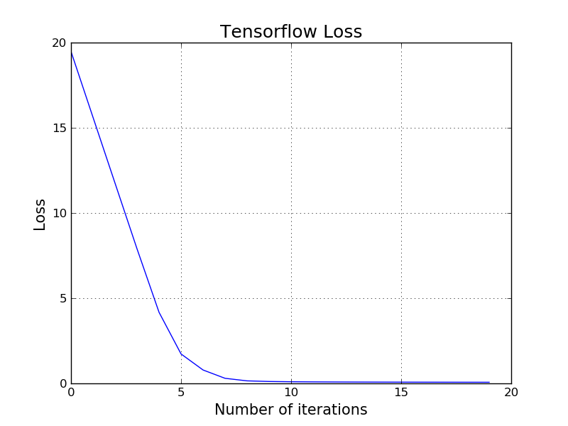
It is maybe worth mentioning that the Logistic Regression we have just built is technically can be considered a Neural Network with only one layer. The techniques and the idea of building Neural Networks is extremely similar to the mechanics of Logistic Regression. More specifically, we define a loss function, we take the derivative of the loss function, we use gradient descent, etc. in Neural Networks as well.
If you are interested learning more about Deep Learning and Neural Networks, you can go start reading Part 2: Softmax Regression.
Appendix
Let's spend some time on the decision of using the sigmoid function and the consequences of it.
Why do we use the sigmoid function?
- Historically popular
- Squashes numbers to range $(0,1)$. This is a nice property since we want to build a binary classifier
- Differentiable in every point
- It has "beautiful" derivatives that makes a nice math (after backpropagation) which produces good $\frac{\partial \text{L}}{\partial \mathbf{w}}$. For example: $\frac{\partial \text{L}}{\partial w_1} = (a-y)x_1$
- The loss surface is convex (if we use MLE)
On the other hand it has problems like vanishing gradients. However, let's skip this for now, and focus more about the convexity.
How do we prove the error surface of logistic regression is convex?
First of all, what is the proper definition of convexity?
Before jumping to that, let's think about another loss function. Say: Sum of squared loss . How would Sum of squared loss behave on the same problem.
Let's remember our loss function we derived using MLE:
$$ \text{L} = -(y\text{log}(a) + (1-y) \text{log}(1-a)) $$which produces a convex surface.
Let's try to use least squared loss instead: $$ \text{L} = (y-a)^2 $$This should look pretty intuitive. If the difference between $y$ and $a$ is big, then the loss is big, and vice versa.
Now, let's see the loss surface for the least squared loss for the same problem.
NX = 100
NY = 100

def get_least_square_loss(X, y, w, b):
  total_loss = 0.0
  for i in range(X.shape[0]):
    x_i = X[i,:]
    z = w.dot(x_i) + b
    a = sigmoid(z)
    total_loss += (y[i] - a) ** 2
  return total_loss / X.shape[0]

xs = np.linspace(-100, 100, NX)
ys = np.linspace(-100, 100, NY)
xv, yv = np.meshgrid(xs, ys)

w_fake = np.stack((xv.flatten(), yv.flatten()), axis=1)

losses = []
for i in range(w_fake.shape[0]):
  losses.append( get_least_square_loss(X, y, w_fake[i,:], b_cache[-1]) )
losses = np.array(losses)

def plot_error_surface(X, y, losses):
  plt.grid()

  fig = plt.figure()
  fig.suptitle('Error surface for Least Squared loss', fontsize=17)
  ax = fig.add_subplot(1, 1, 1, projection='3d')
  ax.set_xlabel('$w_1$', size=20)
  ax.set_ylabel('$w_2$', size=20)
  ax.plot_surface(xv, yv, losses.reshape(NX, NY), rstride=4, cstride=4, alpha=0.25)

  fig.tight_layout()
  plt.savefig('image.png')

plot_error_surface(X, y, losses)

plt.close()
plt.clf()
plt.cla()
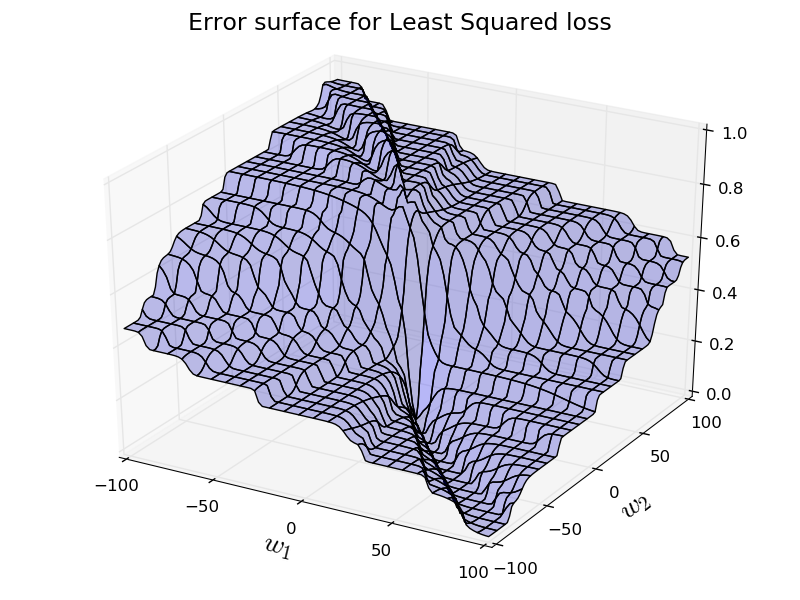
So, the loss surface is not too bad. However, it is not convex anymore. So, we don't have any nice guarantees. Our gradient descent may get stuck at local minimas.
I don't want to write out the all proof for the convexity of MLE, however I will give a sketch of the proof.
Let's remember our loss function for multiple samples:
$$ \text{J} = - \sum_{i=1}^m {y^{(i)}} \text{log} \left( a^{(i)} \right ) + (1-y^{(i)}) \text{log} \left ( 1-a^{(i)} \right ) $$Okay. So, we know that any positive linear combination of two convex functions is convex as well.
This means that if we can prove:
$$ \text{log}(a) = \text{log} \left (\frac{1}{1+e^{\mathbf{w}\mathbf{x} + b}} \right ) $$and
$$ \text{log}(1-a) = \text{log} \left (1 - \frac{1}{1+e^{\mathbf{w}\mathbf{x} + b}} \right ) $$is convex with respect to $\mathbf{w}$ and $b$, then our loss function must be also convex. Because we know that $y \in \{0,1\}$, it is positive linear combination of two convex functions.
One can prove that both of the above functions are convex with respect to $\mathbf{w}$ and $b$ (independently) using the second-order condition of convexity.
High Level Algorithm
Here is the high level code of what we are actually doing. I urge you all to use the same input values I used, and write Logistic Regression from scratch on your own.
It is also a nice practice to derive all the Logistic Regression math from scratch.
Randomly initialize w1 and w2
Randomly initialize b

do NUM_EPOCHS time:
  for x, y in samples:
    compute z = w1 x1 + w2 x2 + b
    compute a = sigmoid(z)
    compute numerically stable loss
    compute derivative of loss w.r.t w_1  (dL/dw1)
    compute derivative of loss w.r.t w_2  (dL/dw2)
    compute derivative of loss w.r.t b    (dL/db)

  print average loss

  w1 := w1 - LEARNING_PARAMETER * average dL/dw1
  w2 := w2 - LEARNING_PARAMETER * average dL/dw2
  b := b - LEARNING_PARAMETER * average dL/b

Predict all points using w_1, w_2, b and compute accuracy
References
- Andrew Ng Coursera Machine Learning course.
- http://cs229.stanford.edu/notes/cs229-notes1.pdf
- http://colah.github.io/posts/2015-08-Backprop/
- http://neuralnetworksanddeeplearning.com/chap2.html
- https://theclevermachine.wordpress.com/2014/09/08/derivation-derivatives-for-common-neural-network-activation-functions/
- http://ufldl.stanford.edu/tutorial/
- https://distill.pub/
- http://cs231n.github.io/
- https://www.youtube.com/watch?v=QWfmCyLEQ8U
- https://www.tensorflow.org/
- http://www.ccs.neu.edu/home/vip/teach/MLcourse/2_GD_REG_pton_NN/lecture_notes/logistic_regression_loss_function/logistic_regression_loss.pdf